Metal Units (Velocity Rescaling)

This notebook demonstrates the use of a unit system (metal units) for the simulation of the Silicon crystal containing 512 atoms with velocity rescaling thermostat and the Stillinger-Weber potential. This notebook use lammps velocities and positions as a starting point for the simulation and for comparison.

More about the unit system https://docs.lammps.org/units.html

Imports & Utils

import os

IN_COLAB = 'COLAB_RELEASE_TAG' in os.environ
if IN_COLAB:
  import subprocess
  import sys

  subprocess.run(
    [
      sys.executable,
      '-m',
      'pip',
      'install',
      '-q',
      'git+https://github.com/jax-md/jax-md.git',
    ]
  )

import jax.numpy as jnp
import numpy as onp
from jax import debug
from jax import jit
from jax import grad
from jax import random
from jax import lax
from jax import config

config.update('jax_enable_x64', True)
from jax_md import simulate
from jax_md import space
from jax_md import energy
from jax_md import elasticity
from jax_md import quantity
from jax_md import dataclasses
from jax_md.util import f64

# Other libraries
import matplotlib
import matplotlib.pyplot as plt
import pandas as pd
from typing import Callable, Tuple, TextIO, Dict, Any, Optional, TypeVar

Download LAMMPS Data

# LAMMPS simulation data for comparison
import urllib.request

SMOKE_TEST = os.environ.get('READTHEDOCS', False)


def download_file(url, filename):
  if not os.path.exists(filename):
    urllib.request.urlretrieve(url, filename)


base_url = 'https://raw.githubusercontent.com/abhijeetgangan/silicon_data/main/Si_FF/Si_SW_MD/NVT_explicit_300K/'
download_file(base_url + 'lammps_nvt.dat', 'velocity_rescale_nvt.dat')

# Download initial positions from NVE simulation
base_url_nve = 'https://raw.githubusercontent.com/abhijeetgangan/silicon_data/main/Si_FF/Si_SW_MD/NVE_300K/'
download_file(base_url_nve + 'step_1.traj', 'step_1.traj')

data_lammps = pd.read_csv(
  'velocity_rescale_nvt.dat', sep=r'\s+', header=None
)
data_lammps = data_lammps.dropna(axis=1)
data_lammps.columns = ['Time', 'T', 'P', 'V', 'E', 'H']
t_l, T_l, P_l, V_l, E_l, H_l = (
  data_lammps['Time'],
  data_lammps['T'],
  data_lammps['P'],
  data_lammps['V'],
  data_lammps['E'],
  data_lammps['H'],
)

Load LAMMPS Positions and Velocities

lammps_step_0 = onp.loadtxt('step_1.traj', dtype=f64)

# Load positions from lammps
positions = jnp.array(lammps_step_0[:, 2:5], dtype=f64)
# Load velocities from lammps
velocity = jnp.array(lammps_step_0[:, 5:8], dtype=f64)
latvec = jnp.array(
  [
    [21.724, 0.000000, 0.000000],
    [0.00000, 21.724, 0.00000],
    [0.00000, 0.0000, 21.724],
  ]
)

Units and Simulation Parameters

# Import unit system
from jax_md import units

# Metal units
unit = units.metal_unit_system()

# Simulation parameters
timestep = 1e-3
fs = timestep * unit['time']
ps = unit['time']
dt = fs
write_every = 100
box = latvec
T_init = 300 * unit['temperature']
Mass = 28.0855 * unit['mass']
key = random.PRNGKey(121)

NSTEPS_SIM = 1000 if SMOKE_TEST else 50000

# Logger to save data
log = {
  'E': jnp.zeros((NSTEPS_SIM // write_every,)),
  'P': jnp.zeros((NSTEPS_SIM // write_every,)),
  'T': jnp.zeros((NSTEPS_SIM // write_every,)),
  'kT': jnp.zeros((NSTEPS_SIM // write_every,)),
}

Simulation Setup

# Setup the periodic boundary conditions.
displacement, shift = space.periodic_general(latvec)
dist_fun = space.metric(displacement)
neighbor_fn, energy_fn = energy.stillinger_weber_neighbor_list(
  displacement, latvec, disable_cell_list=True
)
energy_fn = jit(energy_fn)

# Extra capacity to prevent overflow
nbrs = neighbor_fn.allocate(positions, box=box, extra_capacity=0)

# Velocity rescaling simulation
init_fn, apply_fn = simulate.temp_rescale(
  energy_fn,
  shift,
  dt=dt,
  kT=T_init,
  window=15 * unit['temperature'],
  fraction=0.5,
)
apply_fn = jit(apply_fn)
state = init_fn(key, positions, box=box, neighbor=nbrs, kT=T_init, mass=Mass)

# Restart from LAMMPS velocities
state = dataclasses.replace(state, momentum=Mass * velocity * unit['velocity'])

/home/docs/checkouts/readthedocs.org/user_builds/jax-md/envs/main/lib/python3.12/site-packages/jax/_src/ops/scatter.py:104: FutureWarning: scatter inputs have incompatible types: cannot safely cast value from dtype=int64 to dtype=int32 with jax_numpy_dtype_promotion=standard. In future JAX releases this will result in an error.
  warnings.warn(

Velocity Rescaling Simulation

@jit
def step_fn(i, state_nbrs):
  state, nbrs = state_nbrs
  # Take a simulation step.
  t = i * dt
  state = apply_fn(state, neighbor=nbrs, kT=T_init)
  nbrs = nbrs.update(state.position, neighbor=nbrs)
  return state, nbrs


@jit
def outer_sim_fn(j, state_nbrs_log):
  state, nbrs, log = state_nbrs_log

  # Quantities to calculate
  K = quantity.kinetic_energy(momentum=state.momentum, mass=Mass)
  E = energy_fn(state.position, box=box, neighbor=nbrs)
  kT = quantity.temperature(momentum=state.momentum, mass=Mass)
  P = quantity.pressure(energy_fn, state.position, box, K, neighbor=nbrs)

  # Save the quantities
  log['T'] = log['T'].at[j].set(E + K)
  log['E'] = log['E'].at[j].set(E)
  log['kT'] = log['kT'].at[j].set(kT)
  log['P'] = log['P'].at[j].set(P)

  # Print the quantities
  debug.print(
    'Step = {j} | Total Energy = {T} | Temp = {Temp}',
    j=j * write_every,
    T=E,
    Temp=kT / unit['temperature'],
  )

  @jit
  def inner_sim_fn(i, state_nbrs):
    return step_fn(i, state_nbrs)

  state, nbrs = lax.fori_loop(0, write_every, inner_sim_fn, (state, nbrs))

  return state, nbrs, log

state_r, nbrs_r, log_r = lax.fori_loop(
  0, int(NSTEPS_SIM / write_every), outer_sim_fn, (state, nbrs, log)
)

Step = 0 | Total Energy = -2220.2982374604026 | Temp = 299.414519001463
Step = 100 | Total Energy = -2202.1338212916244 | Temp = 304.43927341983346
Step = 200 | Total Energy = -2199.5814292854493 | Temp = 297.4465849105166
Step = 300 | Total Energy = -2198.3192132759546 | Temp = 286.8765431122266
Step = 400 | Total Energy = -2198.2398137535733 | Temp = 283.7501684183033
Step = 500 | Total Energy = -2201.4791594058725 | Temp = 284.9618503964879
Step = 600 | Total Energy = -2200.458475511886 | Temp = 317.04257305984675
Step = 700 | Total Energy = -2199.5515397609324 | Temp = 280.43011413619143
Step = 800 | Total Energy = -2201.9410533072105 | Temp = 312.1591166466383
Step = 900 | Total Energy = -2199.6755065151024 | Temp = 306.3911345009189

# Check if neighbors overflowed
print(nbrs_r.did_buffer_overflow)

0

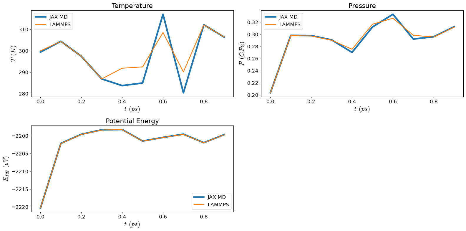
Comparison Plot

NSTEPS = int(NSTEPS_SIM / write_every)
t = jnp.arange(0, NSTEPS, dtype=f64) * timestep * write_every

matplotlib.rcParams['mathtext.fontset'] = 'cm'
matplotlib.rcParams.update({'font.size': 12})
fig = plt.figure(figsize=(16, 8))

ax1 = plt.subplot(2, 2, 1)
ax1.plot(t, log_r['kT'] / unit['temperature'], lw=4, label='JAX MD')
if data_lammps is not None:
  ax1.plot(t_l[:NSTEPS], T_l[:NSTEPS], lw=2, label='LAMMPS')
ax1.set_title('Temperature', fontsize=16)
ax1.set_ylabel('$T\\ (K)$', fontsize=16)
ax1.set_xlabel('$t\\ (ps)$', fontsize=16)
ax1.legend()

ax2 = plt.subplot(2, 2, 2)
ax2.plot(t, (log_r['P'] / unit['pressure']) / 10000, lw=4, label='JAX MD')
if data_lammps is not None:
  ax2.plot(t_l[:NSTEPS], P_l[:NSTEPS] / 10000, lw=2, label='LAMMPS')
ax2.set_title('Pressure', fontsize=16)
ax2.set_ylabel('$P\\ (GPa)$', fontsize=16)
ax2.set_xlabel('$t\\ (ps)$', fontsize=16)
ax2.legend()

ax3 = plt.subplot(2, 2, 3)
ax3.plot(t, log_r['E'], lw=4, label='JAX MD')
if data_lammps is not None:
  ax3.plot(t_l[:NSTEPS], E_l[:NSTEPS], lw=2, label='LAMMPS')
ax3.set_title('Potential Energy', fontsize=16)
ax3.set_ylabel('$E_{PE}\\ (eV)$', fontsize=16)
ax3.set_xlabel('$t\\ (ps)$', fontsize=16)
ax3.legend()

fig.tight_layout()
plt.show()

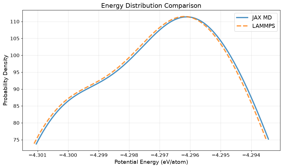
Energy Distribution Comparison

Compare the distribution of potential energies between JAX-MD and LAMMPS

from scipy import stats

# Skip first few points for equilibration
NSKIP = 1

# Calculate KDE for smooth distribution
jax_energy = onp.array(log_r['E'][NSKIP:] / 512)
kde_jax = stats.gaussian_kde(jax_energy)
x_range = onp.linspace(jax_energy.min(), jax_energy.max(), 200)

plt.figure(figsize=(10, 6))
plt.plot(x_range, kde_jax(x_range), linewidth=3, label='JAX MD', alpha=0.8)

if data_lammps is not None:
  lammps_energy = onp.array(E_l[NSKIP:NSTEPS] / 512)
  kde_lammps = stats.gaussian_kde(lammps_energy)
  x_range_lammps = onp.linspace(lammps_energy.min(), lammps_energy.max(), 200)
  plt.plot(
    x_range_lammps,
    kde_lammps(x_range_lammps),
    linewidth=3,
    label='LAMMPS',
    alpha=0.8,
    linestyle='--',
  )

plt.xlabel('Potential Energy (eV/atom)', fontsize=14)
plt.ylabel('Probability Density', fontsize=14)
plt.title('Energy Distribution Comparison', fontsize=16)
plt.legend(fontsize=14)
plt.grid(True, alpha=0.3)
plt.tight_layout()
plt.show()