Neural Network Potentials

An area of significant recent interest is the use of neural networks to model quantum mechanics. Since directly solving Schrodinger’s equation is extremely expensive, these techniques offer the possibility of conducting large-scale and high-fidelity experiments of materials as well as chemical and biochemical systems.

Here we will use a Graph Neural Network (GNN) to learn a potential for a 64-atom Silicon system. The dataset comes from DFT simulations at 300K, 600K, and 900K in several crystal phases. We will train on energies and forces, and then use the learned potential to run an NVT molecular dynamics simulation.

Imports & Utils

import os
import pickle
import tempfile
from functools import partial
from pathlib import Path
import json
import urllib.request
import ase.db

IN_COLAB = 'COLAB_RELEASE_TAG' in os.environ
if IN_COLAB:
  import subprocess
  import sys

  subprocess.run(
    [
      sys.executable,
      '-m',
      'pip',
      'install',
      '-q',
      'git+https://github.com/jax-md/jax-md.git',
      'optax',
    ]
  )

import warnings

warnings.simplefilter('ignore')

from flax import nnx
import jax
import jax.numpy as np
from jax import grad
from jax import jit
from jax import lax
from jax import random
from jax import vmap
import matplotlib.pyplot as plt
import numpy as onp
import optax
import seaborn as sns

from jax_md import energy, nn, quantity, simulate, space, units
from jax_md._nn.util import convert_checkpoint_to_params

SMOKE_TEST = os.environ.get('READTHEDOCS', False)

CHECKPOINT_URL = (
  'https://raw.githubusercontent.com/google/jax-md/main/examples/models/'
  'si_gnn.pickle'
)
SILICON_DATA_BASE_URL = (
  'https://raw.githubusercontent.com/abhijeetgangan/silicon_data/main/'
  'Si_DFT/silicon_aselmdb/'
)

CACHE_DIR = Path(tempfile.gettempdir()) / 'jax_md_neural_networks'
CHECKPOINT_PATH = CACHE_DIR / 'si_gnn.pickle'
ASELMDB_CACHE = CACHE_DIR / 'silicon_aselmdb'

NO_SKIP = 80 if SMOKE_TEST else 15
MAX_SHARDS = 2 if SMOKE_TEST else None
TRAIN_EPOCHS = 2 if SMOKE_TEST else 20
N_PREDICTIONS = 64 if SMOKE_TEST else 500
FORCE_EVAL_COUNT = 32 if SMOKE_TEST else 300
SIMULATION_STEPS = 100 if SMOKE_TEST else 10000
SIMULATION_PRINT_EVERY = 1 if SMOKE_TEST else 40
SIMULATION_WRITE_EVERY = 25
BATCH_SIZE = 4 if SMOKE_TEST else 128

sns.set_style(style='white')
sns.set(font_scale=1.6)


def format_plot(x, y):
  plt.xlabel(x, fontsize=20)
  plt.ylabel(y, fontsize=20)


def finalize_plot(shape=(1, 1)):
  plt.gcf().set_facecolor('white')
  plt.gcf().set_size_inches(
    shape[0] * 1.5 * plt.gcf().get_size_inches()[1],
    shape[1] * 1.5 * plt.gcf().get_size_inches()[1],
  )
  plt.tight_layout()


def download_file(url, path):
  path.parent.mkdir(parents=True, exist_ok=True)
  if path.exists():
    return path
  print(f'Downloading {url} -> {path}')
  urllib.request.urlretrieve(url, path)
  return path


def shard_indices_for_phases(manifest, phases):
  shard_size = manifest['shard_size']
  offset = 0
  first_frame = None
  last_frame = None
  for source_name in sorted(manifest['source_counts']):
    count = manifest['source_counts'][source_name]
    phase = source_name.replace('MD_DATA.', '', 1)
    if phase in phases:
      if first_frame is None:
        first_frame = offset
      last_frame = offset + count - 1
    offset += count
  if first_frame is None:
    return set()
  return set(range(first_frame // shard_size, last_frame // shard_size + 1))


def ensure_silicon_aselmdb(phases=('cubic_300K', 'cubic_600K', 'cubic_900K')):
  ASELMDB_CACHE.mkdir(parents=True, exist_ok=True)
  manifest_path = ASELMDB_CACHE / 'manifest.json'
  download_file(SILICON_DATA_BASE_URL + 'manifest.json', manifest_path)
  with manifest_path.open() as f:
    manifest = json.load(f)
  needed = sorted(shard_indices_for_phases(manifest, set(phases)))
  if MAX_SHARDS is not None:
    needed = needed[:MAX_SHARDS]
  for idx in needed:
    name = f'data_{idx:04d}.aselmdb'
    download_file(SILICON_DATA_BASE_URL + name, ASELMDB_CACHE / name)
  return ASELMDB_CACHE


def ensure_silicon_assets():
  CACHE_DIR.mkdir(parents=True, exist_ok=True)
  download_file(CHECKPOINT_URL, CHECKPOINT_PATH)
  aselmdb_dir = ensure_silicon_aselmdb()
  return CHECKPOINT_PATH, aselmdb_dir


def draw_training_summary(params):
  plt.figure()
  plt.subplot(1, 2, 1)
  plt.semilogy(train_energy_error)
  plt.semilogy(test_energy_error)
  plt.xlim([0, train_epochs])
  format_plot('Epoch', '$L$')
  plt.subplot(1, 2, 2)
  predicted = vectorized_energy_fn(params, example_positions)
  plt.plot(example_energies, predicted, 'o')
  plt.plot(np.linspace(-400, -300, 10), np.linspace(-400, -300, 10), '--')
  format_plot('$E_{label}$', '$E_{prediction}$')
  finalize_plot((2, 1))
  plt.show()


def aselmdb_shards(aselmdb_dir):
  shards = sorted(aselmdb_dir.glob('data_*.aselmdb'))
  if not shards:
    raise FileNotFoundError(f'No `.aselmdb` shards found in {aselmdb_dir}.')
  return shards


def load_lmdb_samples(aselmdb_dir, phases, no_skip=20):
  stride = max(int(no_skip), 1)
  phase_counts = {phase: 0 for phase in phases}
  positions = []
  forces = []
  energies = []

  for shard_path in aselmdb_shards(aselmdb_dir):
    with ase.db.connect(shard_path) as db:
      for row in db.select():
        phase = row.data.get('phase')
        if phase not in phase_counts:
          continue
        if phase_counts[phase] % stride == 0:
          positions.append(onp.asarray(row.positions))
          forces.append(onp.asarray(row.forces))
          energies.append(float(row.energy))
        phase_counts[phase] += 1

  if not positions:
    raise ValueError(f'No matching samples found in {aselmdb_dir}.')

  return np.array(positions), np.array(energies), np.array(forces)


def build_dataset(aselmdb_dir):
  all_data, all_energies, all_forces = load_lmdb_samples(
    aselmdb_dir,
    phases=('cubic_300K', 'cubic_600K', 'cubic_900K'),
    no_skip=NO_SKIP,
  )
  total_samples = all_data.shape[0]

  onp.random.seed(0)
  lookup = onp.random.permutation(range(total_samples))
  all_data = all_data[lookup]
  all_energies = all_energies[lookup]
  all_forces = all_forces[lookup]

  train_count = int(total_samples * 0.65)
  train_data = all_data[:train_count]
  test_data = all_data[train_count:]
  train_energies = all_energies[:train_count]
  test_energies = all_energies[train_count:]
  train_forces = all_forces[:train_count]
  test_forces = all_forces[train_count:]

  return (
    (train_data, train_energies, train_forces),
    (test_data, test_energies, test_forces),
  )

Download Data

The pretrained checkpoint and the silicon .aselmdb shards are cached from the shared abhijeetgangan/silicon_data GitHub repository.

checkpoint_path, aselmdb_dir = ensure_silicon_assets()
print(f'Using silicon dataset at {aselmdb_dir}')

Downloading https://raw.githubusercontent.com/google/jax-md/main/examples/models/si_gnn.pickle -> /tmp/jax_md_neural_networks/si_gnn.pickle
Downloading https://raw.githubusercontent.com/abhijeetgangan/silicon_data/main/Si_DFT/silicon_aselmdb/manifest.json -> /tmp/jax_md_neural_networks/silicon_aselmdb/manifest.json
Downloading https://raw.githubusercontent.com/abhijeetgangan/silicon_data/main/Si_DFT/silicon_aselmdb/data_0020.aselmdb -> /tmp/jax_md_neural_networks/silicon_aselmdb/data_0020.aselmdb
Downloading https://raw.githubusercontent.com/abhijeetgangan/silicon_data/main/Si_DFT/silicon_aselmdb/data_0021.aselmdb -> /tmp/jax_md_neural_networks/silicon_aselmdb/data_0021.aselmdb
Using silicon dataset at /tmp/jax_md_neural_networks/silicon_aselmdb

Build the Dataset

We load the data into training and test sets. Each split includes particle positions, whole-system energies, and per-particle forces. To assist in training we compute the mean and standard deviation of the data and use this to set the initial scale for our neural network.

train, test = build_dataset(aselmdb_dir)

positions, energies, forces = train
test_positions, test_energies, test_forces = test

energy_mean = np.mean(energies)
energy_std = np.std(energies)

print(f'positions.shape = {positions.shape}')
print(f'<E> = {energy_mean}')
print(f'std(E) = {energy_std}')

positions.shape = (16, 64, 3)
<E> = -379.997314453125
std(E) = 1.466552495956421

Define the Periodic Space

We create a space for our systems to live in using periodic boundary conditions.

box_size = 10.862
displacement, shift = space.periodic(box_size)

Construct the Graph Network

We instantiate a graph neural network using energy.graph_network_neighbor_list. This neural network is based on recent work modelling defects in disordered solids. See that paper or the review by Battaglia et al. for details. We add edges between all neighbors separated by less than a cutoff of 3 Angstroms. The function returns (neighbor_fn, energy_fn) matching the same convention as lennard_jones_neighbor_list etc.

key = random.PRNGKey(0)
neighbor_fn, energy_fn = energy.graph_network_neighbor_list(
  displacement, box_size, r_cutoff=3.0, dr_threshold=0.0, key=key
)
nnx.display(energy_fn.model)

Allocate a Neighbor Prototype

We construct an initial neighbor list which will be used to estimate the maximum number of neighbors. This is necessary since XLA needs to have static shapes to enable JIT compilation.

neighbor = neighbor_fn.allocate(positions[0], extra_capacity=6)
print(f'Allocating space for at most {neighbor.idx.shape[-1]} edges')

Allocating space for at most 784 edges

Define Energy and Force Functions

Using the neighbor prototype we write wrappers around the energy function that construct a neighbor list for a given state and then compute the energy. This allows us to use JAX’s automatic vectorization via vmap along with our neighbor lists. Using JAX’s automatic differentiation we can also write down a function that computes the force due to our neural network potential.

Note that if we were running a simulation using this energy, we would only rebuild the neighbor list when necessary.

For training with vmap/grad/optax we decompose the model into a graphdef and state via nnx.split and use the graphdef.apply(state) functional forward pass.

graphdef, state = nnx.split(energy_fn.model)
init_params = state
params = init_params


def apply(state, *args, **kwargs):
  out, _ = graphdef.apply(state)(*args, **kwargs)
  return out


def train_energy(params, R):
  return apply(params, R, neighbor.update(R))


vectorized_energy_fn = jit(vmap(train_energy, (None, 0)))
vectorized_force_fn = jit(vmap(
  lambda params, R: -grad(train_energy, argnums=1)(params, R), (None, 0)
))

Plot Untrained Predictions

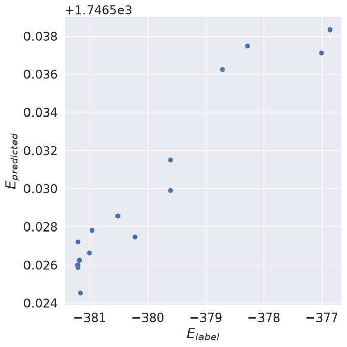
We can compute predicted energies for all states using the untrained network. Despite being untrained, the outputs of the graph network correlate with the labels – hinting that graph networks provide some sort of “deep molecular prior”.

example_count = min(N_PREDICTIONS, positions.shape[0])
example_positions = positions[:example_count]
example_energies = energies[:example_count]
example_forces = forces[:example_count]

predicted = vectorized_energy_fn(params, example_positions)

plt.plot(example_energies, predicted, 'o')
format_plot('$E_{label}$', '$E_{predicted}$')
finalize_plot((1, 1))
plt.show()

Define Losses

We define losses for the energy and the force as well as a total loss that combines the two terms. We fit both using Mean-Squared-Error (MSE) loss.

@jit
def energy_loss(params, R, energy_targets):
  return np.mean((vectorized_energy_fn(params, R) - energy_targets) ** 2)


@jit
def force_loss(params, R, force_targets):
  dforces = vectorized_force_fn(params, R) - force_targets
  return np.mean(np.sum(dforces ** 2, axis=(1, 2)))


@jit
def loss(params, R, targets):
  return energy_loss(params, R, targets[0]) + force_loss(params, R, targets[1])

Optimizer

We create an optimizer using Adam with gradient clipping and write helper functions to perform a single update step and an entire epoch of updates.

opt = optax.chain(optax.clip_by_global_norm(1.0), optax.adam(1e-3))


@jit
def update_step(params, opt_state, R, labels):
  updates, opt_state = opt.update(grad(loss)(params, R, labels), opt_state)
  return optax.apply_updates(params, updates), opt_state


@jit
def update_epoch(params_and_opt_state, batches):
  def inner_update(params_and_opt_state, batch):
    params, opt_state = params_and_opt_state
    batch_positions, batch_labels = batch
    return update_step(params, opt_state, batch_positions, batch_labels), 0

  return lax.scan(inner_update, params_and_opt_state, batches)[0]

We also write a function that creates an epoch’s worth of batches given a lookup table that shuffles all of the states in the training set.

def make_batches(lookup):
  batch_positions = []
  batch_energies = []
  batch_forces = []

  for start in range(0, len(lookup), BATCH_SIZE):
    stop = start + BATCH_SIZE
    if stop > len(lookup):
      break
    idx = lookup[start:stop]
    batch_positions.append(positions[idx])
    batch_energies.append(energies[idx])
    batch_forces.append(forces[idx])

  return np.stack(batch_positions), np.stack(batch_energies), np.stack(batch_forces)

Train Briefly

We train for twenty epochs to make sure the network starts learning.

train_epochs = TRAIN_EPOCHS
opt_state = opt.init(params)

train_energy_error = []
test_energy_error = []

lookup = onp.arange(positions.shape[0])
onp.random.shuffle(lookup)
batch_positions, batch_energies, batch_forces = make_batches(lookup)

for _ in range(train_epochs):
  train_energy_error.append(
    float(np.sqrt(energy_loss(params, batch_positions[0], batch_energies[0])))
  )
  test_energy_error.append(
    float(np.sqrt(energy_loss(params, test_positions, test_energies)))
  )

  params, opt_state = update_epoch(
    (params, opt_state),
    (batch_positions, (batch_energies, batch_forces)),
  )

  onp.random.shuffle(lookup)
  batch_positions, batch_energies, batch_forces = make_batches(lookup)

draw_training_summary(params)

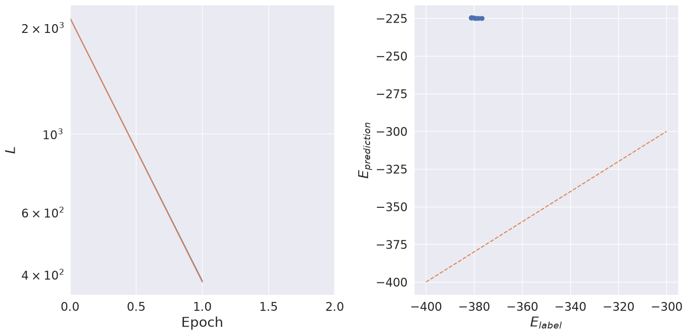
While we see that the network has begun to learn the energies, we also see that it has a long way to go before the predictions get good enough to use in a simulation. As such we take inspiration from cooking shows, and take a ready-made GNN out of the fridge where it has been training overnight for 12,000 epochs on a V100 GPU.

with checkpoint_path.open('rb') as f:
  raw_checkpoint_params = pickle.load(f)

init_pure = nnx.to_pure_dict(init_params)
converted_pure = convert_checkpoint_to_params(raw_checkpoint_params, init_pure)
nnx.replace_by_pure_dict(params, converted_pure)

Plot Pretrained Energy and Force Predictions

Using the trained model we plot predicted energies and forces against labels.

force_eval_count = min(FORCE_EVAL_COUNT, test_positions.shape[0])

plt.figure()
plt.subplot(1, 2, 1)

predicted_energies = vectorized_energy_fn(params, example_positions)
plt.plot(example_energies, predicted_energies, 'o')
format_plot('$E_{label}$', '$E_{predicted}$')

plt.subplot(1, 2, 2)

predicted_forces = vectorized_force_fn(params, test_positions[:force_eval_count])
plt.plot(
  test_forces[:force_eval_count].reshape((-1,)),
  predicted_forces.reshape((-1,)),
  'o',
)
plt.plot(np.linspace(-6, 6, 20), np.linspace(-6, 6, 20), '--')
plt.xlim([-5, 5])
plt.ylim([-5, 5])

format_plot('$F_{label}$', '$F_{predicted}$')
finalize_plot((2, 1))
plt.show()

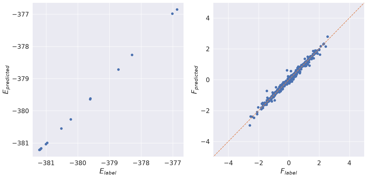
Compute Energy RMSE

We see that the model prediction for the energy is extremely accurate and the force prediction is reasonable. To make this a bit more quantitative, we compute the RMSE of the energy and convert it to meV / atom.

rmse = energy_loss(params, test_positions, test_energies) * 1000 / 64
print(f'RMSE Error of {rmse:.02f} meV / atom')

RMSE Error of 0.01 meV / atom

Build an NVT Simulation

We get an error of about 2 meV / atom, which is comparable to previous work on this system.

Now that we have a well-performing neural network, we can see how easily this network can be used to run a simulation approximating Silicon. We will run a constant temperature simulation using a Nose-Hoover thermostat.

def E_fn(R, neighbor=None, **kwargs):
  return apply(params, R, neighbor, **kwargs)

metal = units.metal_unit_system()
kB = metal['temperature']
dt = 1e-3 * metal['time']
kT = kB * 300
Si_mass = 28.0855 * metal['mass']

sim_init_fn, sim_apply_fn = simulate.nvt_nose_hoover(E_fn, shift, dt, kT)
sim_apply_fn = jit(sim_apply_fn)

Run the Simulation

We run the simulation for 10,000 steps while writing the energy and temperature throughout.

total_steps = SIMULATION_STEPS
steps_per_recording = SIMULATION_WRITE_EVERY
total_records = total_steps // steps_per_recording


@jit
def sim(state, nbrs):
  def step(_, state_and_nbrs):
    state, nbrs = state_and_nbrs
    nbrs = nbrs.update(state.position)
    return sim_apply_fn(state, neighbor=nbrs), nbrs

  return lax.fori_loop(0, steps_per_recording, step, (state, nbrs))


nbrs = neighbor_fn.allocate(test_positions[0], extra_capacity=6)
state = sim_init_fn(key, test_positions[0], Si_mass, neighbor=nbrs)

simulation_positions = []

print('Energy (eV)\tTemperature (K)')
for i in range(total_records):
  state, nbrs = sim(state, nbrs)
  simulation_positions.append(state.position)

  if i % SIMULATION_PRINT_EVERY == 0:
    print(
      '{:.02f}\t\t\t{:.02f}'.format(
        E_fn(state.position, neighbor=nbrs),
        quantity.temperature(momentum=state.momentum, mass=Si_mass) / kB,
      )
    )

simulation_positions = np.stack(simulation_positions)

Energy (eV)     Temperature (K)
-377.73                 369.86
-378.27                 413.55
-378.55                 407.60
-378.07                 320.01

Visualize the Final Configuration

We see that the energy of the simulation is reasonable and the temperature is stable. Of course, if we were validating this model for use in a research setting there are many measurements that one would like to perform to check its fidelity.

We can now draw the simulation to see what is happening.

if IN_COLAB:
  from jax_md.colab_tools import renderer

  nbrs = nbrs.update(state.position)
  renderer.render(
    box_size,
    {
      'atom': renderer.Sphere(simulation_positions),
      'bonds': renderer.Bond('atom', nbrs.idx),
    },
    resolution=[512, 512],
  )