Metal Units (NVE Simulation)

This notebook demonstrates the use of a unit system (metal units) for the simulation of the Silicon crystal containing 512 atoms in the NVE ensemble with the Stillinger-Weber potential. This notebook use lammps velocities and positions as a starting point for the simulation and for comparison.

More about the unit system https://docs.lammps.org/units.html

Imports & Utils

import os

IN_COLAB = 'COLAB_RELEASE_TAG' in os.environ
if IN_COLAB:
  import subprocess
  import sys

  subprocess.run(
    [
      sys.executable,
      '-m',
      'pip',
      'install',
      '-q',
      'git+https://github.com/jax-md/jax-md.git',
    ]
  )

import jax.numpy as jnp
import numpy as onp
from jax import debug
from jax import jit
from jax import grad
from jax import random
from jax import lax
from jax import config

config.update('jax_enable_x64', True)
from jax_md import simulate
from jax_md import space
from jax_md import energy
from jax_md import elasticity
from jax_md import quantity
from jax_md import dataclasses
from jax_md.util import f64

# Other libraries
import matplotlib
import matplotlib.pyplot as plt
import pandas as pd

Download LAMMPS Data

# LAMMPS simulation data for comparison
import urllib.request

SMOKE_TEST = os.environ.get('READTHEDOCS', False)


def download_file(url, filename):
  if not os.path.exists(filename):
    urllib.request.urlretrieve(url, filename)


base_url = 'https://raw.githubusercontent.com/abhijeetgangan/silicon_data/main/Si_FF/Si_SW_MD/NVE_300K/'
download_file(base_url + 'lammps_nve.dat', 'lammps_nve.dat')
download_file(base_url + 'step_1.traj', 'step_1.traj')

data_lammps = pd.read_csv('lammps_nve.dat', sep=r'\s+', header=None)
data_lammps = data_lammps.dropna(axis=1)
data_lammps.columns = ['Time', 'T', 'P', 'V', 'E', 'H']
t_l, T, P, V, E, H = (
  data_lammps['Time'],
  data_lammps['T'],
  data_lammps['P'],
  data_lammps['V'],
  data_lammps['E'],
  data_lammps['H'],
)

Load LAMMPS Positions and Velocities

lammps_step_0 = onp.loadtxt('step_1.traj', dtype=f64)

# Load positions from lammps
positions = jnp.array(lammps_step_0[:, 2:5], dtype=f64)
# Load velocities from lammps
velocity = jnp.array(lammps_step_0[:, 5:8], dtype=f64)
latvec = jnp.array(
  [
    [21.724, 0.000000, 0.000000],
    [0.00000, 21.724, 0.00000],
    [0.00000, 0.0000, 21.724],
  ]
)

Units and Simulation Parameters

# Import unit system
from jax_md import units

# Metal units
unit = units.metal_unit_system()

# Simulation parameters
timestep = 1e-3
fs = timestep * unit['time']
ps = unit['time']
dt = fs
write_every = 100
box = latvec
T_init = 300 * unit['temperature']
Mass = 28.0855 * unit['mass']
key = random.PRNGKey(121)

NSTEPS_SIM = 1500 if SMOKE_TEST else 50000

# Logger to save data
log = {
  'E': jnp.zeros((NSTEPS_SIM // write_every,)),
  'P': jnp.zeros((NSTEPS_SIM // write_every,)),
  'T': jnp.zeros((NSTEPS_SIM // write_every,)),
  'kT': jnp.zeros((NSTEPS_SIM // write_every,)),
}

Simulation Setup

# Setup the periodic boundary conditions.
displacement, shift = space.periodic_general(latvec)
dist_fun = space.metric(displacement)
neighbor_fn, energy_fn = energy.stillinger_weber_neighbor_list(
  displacement, latvec, disable_cell_list=True
)
energy_fn = jit(energy_fn)

# Extra capacity to prevent overflow
nbrs = neighbor_fn.allocate(positions, box=box, extra_capacity=2)

# NVE simulation
init_fn, apply_fn = simulate.nve(energy_fn, shift, dt=dt)
apply_fn = jit(apply_fn)
state = init_fn(key, positions, box=box, neighbor=nbrs, kT=T_init, mass=Mass)

# Restart from LAMMPS velocities
state = dataclasses.replace(state, momentum=Mass * velocity * unit['velocity'])

/home/docs/checkouts/readthedocs.org/user_builds/jax-md/envs/main/lib/python3.12/site-packages/jax/_src/ops/scatter.py:104: FutureWarning: scatter inputs have incompatible types: cannot safely cast value from dtype=int64 to dtype=int32 with jax_numpy_dtype_promotion=standard. In future JAX releases this will result in an error.
  warnings.warn(

NVE Simulation

@jit
def step_fn(i, state_nbrs):
  state, nbrs = state_nbrs
  # Take a simulation step.
  t = i * dt
  state = apply_fn(state, neighbor=nbrs)
  nbrs = nbrs.update(state.position, neighbor=nbrs)
  return state, nbrs


@jit
def outer_sim_fn(j, state_nbrs_log):
  state, nbrs, log = state_nbrs_log

  # Quantities to calculate
  K = quantity.kinetic_energy(momentum=state.momentum, mass=Mass)
  E = energy_fn(state.position, box=box, neighbor=nbrs)
  kT = quantity.temperature(momentum=state.momentum, mass=Mass)
  P = quantity.pressure(energy_fn, state.position, box, K, neighbor=nbrs)

  # Save the quantities
  log['T'] = log['T'].at[j].set(K + E)
  log['E'] = log['E'].at[j].set(E)
  log['kT'] = log['kT'].at[j].set(kT)
  log['P'] = log['P'].at[j].set(P)

  # Print the quantities
  debug.print('Step = {j} | Total Energy = {T}', j=j * write_every, T=K + E)

  @jit
  def inner_sim_fn(i, state_nbrs):
    return step_fn(i, state_nbrs)

  state, nbrs = lax.fori_loop(0, write_every, inner_sim_fn, (state, nbrs))

  return state, nbrs, log

state_r, nbrs_r, log_r = lax.fori_loop(
  0, int(NSTEPS_SIM / write_every), outer_sim_fn, (state, nbrs, log)
)

Step = 0 | Total Energy = -2200.4826561382038
Step = 100 | Total Energy = -2200.46425361738
Step = 200 | Total Energy = -2200.4632203518704
Step = 300 | Total Energy = -2200.4673715115377
Step = 400 | Total Energy = -2200.4657508762048
Step = 500 | Total Energy = -2200.468144031352
Step = 600 | Total Energy = -2200.4680987055954
Step = 700 | Total Energy = -2200.463647099563
Step = 800 | Total Energy = -2200.4687565957956
Step = 900 | Total Energy = -2200.46636327141
Step = 1000 | Total Energy = -2200.4644761826603
Step = 1100 | Total Energy = -2200.4686575463097
Step = 1200 | Total Energy = -2200.468402949992
Step = 1300 | Total Energy = -2200.466480631267
Step = 1400 | Total Energy = -2200.467119464217

# Check if neighbors overflowed
print(nbrs_r.did_buffer_overflow)

0

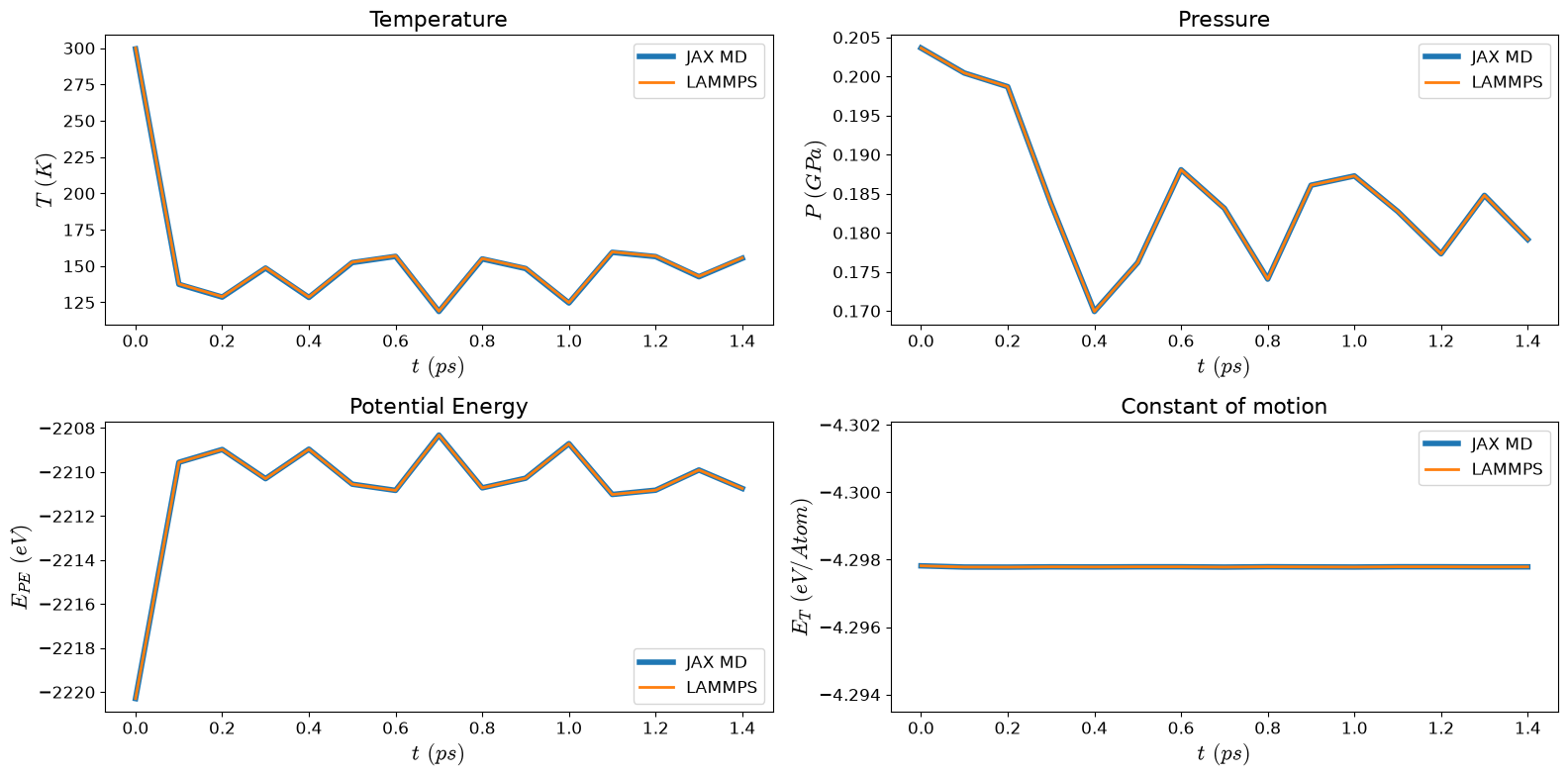
Comparison Plot

Note that you have to reconvert the units again.

NSTEPS = int(NSTEPS_SIM / write_every)
print(NSTEPS)
t = jnp.arange(0, NSTEPS, dtype=f64) * timestep * write_every

15

matplotlib.rcParams['mathtext.fontset'] = 'cm'
matplotlib.rcParams.update({'font.size': 12})
fig = plt.figure(figsize=(16, 8))

ax1 = plt.subplot(2, 2, 1)
ax1.plot(t, log_r['kT'] / unit['temperature'], lw=4, label='JAX MD')
if data_lammps is not None:
  ax1.plot(t_l[:NSTEPS], T[:NSTEPS], lw=2, label='LAMMPS')
ax1.set_title('Temperature', fontsize=16)
ax1.set_ylabel('$T\\ (K)$', fontsize=16)
ax1.set_xlabel('$t\\ (ps)$', fontsize=16)
ax1.legend()

ax2 = plt.subplot(2, 2, 2)
ax2.plot(t, (log_r['P'] / unit['pressure']) / 10000, lw=4, label='JAX MD')
if data_lammps is not None:
  ax2.plot(t_l[:NSTEPS], P[:NSTEPS] / 10000, lw=2, label='LAMMPS')
ax2.set_title('Pressure', fontsize=16)
ax2.set_ylabel('$P\\ (GPa)$', fontsize=16)
ax2.set_xlabel('$t\\ (ps)$', fontsize=16)
ax2.legend()

ax3 = plt.subplot(2, 2, 3)
ax3.plot(t, log_r['E'], lw=4, label='JAX MD')
if data_lammps is not None:
  ax3.plot(t_l[:NSTEPS], E[:NSTEPS], lw=2, label='LAMMPS')
ax3.set_title('Potential Energy', fontsize=16)
ax3.set_ylabel('$E_{PE}\\ (eV)$', fontsize=16)
ax3.set_xlabel('$t\\ (ps)$', fontsize=16)
ax3.legend()

ax4 = plt.subplot(2, 2, 4)
ax4.plot(t, log_r['T'] / 512, lw=4, label='JAX MD')
if data_lammps is not None:
  ax4.plot(t_l[:NSTEPS], H[:NSTEPS] / 512, lw=2, label='LAMMPS')
ax4.set_title('Constant of motion', fontsize=16)
ax4.set_ylabel('$E_{T}\\ (eV/Atom)$', fontsize=16)
ax4.set_xlabel('$t\\ (ps)$', fontsize=16)
ax4.set_ylim(
  jnp.mean(log_r['T'] / 512) - jnp.mean(log_r['T'] / 512) / 1000,
  jnp.mean(log_r['T'] / 512) + jnp.mean(log_r['T'] / 512) / 1000,
)
ax4.legend()

fig.tight_layout()
plt.show()

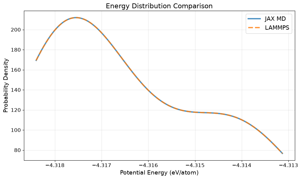
Energy Distribution Comparison

Compare the distribution of total energies between JAX-MD and LAMMPS

from scipy import stats

# Skip first few points for equilibration
NSKIP = 1

# Calculate KDE for smooth distribution
jax_energy = onp.array(log_r['E'][NSKIP:] / 512)
kde_jax = stats.gaussian_kde(jax_energy)
x_range = onp.linspace(jax_energy.min(), jax_energy.max(), 200)

plt.figure(figsize=(10, 6))
plt.plot(x_range, kde_jax(x_range), linewidth=3, label='JAX MD', alpha=0.8)

if data_lammps is not None:
  lammps_energy = onp.array(E[NSKIP:NSTEPS] / 512)
  kde_lammps = stats.gaussian_kde(lammps_energy)
  x_range_lammps = onp.linspace(lammps_energy.min(), lammps_energy.max(), 200)
  plt.plot(
    x_range_lammps,
    kde_lammps(x_range_lammps),
    linewidth=3,
    label='LAMMPS',
    alpha=0.8,
    linestyle='--',
  )

plt.xlabel('Potential Energy (eV/atom)', fontsize=14)
plt.ylabel('Probability Density', fontsize=14)
plt.title('Energy Distribution Comparison', fontsize=16)
plt.legend(fontsize=14)
plt.grid(True, alpha=0.3)
plt.tight_layout()
plt.show()