Symmetric Molecular Dynamics (SyMD)

This example demonstrates how to set up and run a symmetry-constrained molecular dynamics simulation using SyMD and JAX MD. The system is a 2D periodic Lennard-Jones fluid where particles obey a crystallographic space group at every time step.

The workflow:

1. Initialize an asymmetric unit and generate symmetric images

2. FIRE minimization to relax overlaps

3. NVT simulation with symmetry-preserving folding each step

Imports

import os

import jax
jax.config.update('jax_enable_x64', True)

from symd import symd, groups

import jax.numpy as jnp
from jax import random, jit, lax

import matplotlib.pyplot as plt

from jax_md import quantity, space, energy, simulate, minimize, dataclasses

SMOKE_TEST = os.environ.get('READTHEDOCS', False)

Setup a Symmetric System

We load a 2D planar group (Hall number 11) and build the asymmetric-unit constraint function.

GROUP_ID = 11
N = 200 if SMOKE_TEST else 1000
dim = 2

group = groups.load_group(GROUP_ID, dim)
in_unit = symd.asymm_constraints(group.asymm_unit)

Randomly initialize positions in the asymmetric unit and velocities.

key = random.PRNGKey(0)
key, pos_key, vel_key = random.split(key, 3)
pos_key, vel_key = random.split(random.PRNGKey(0))
positions = random.uniform(pos_key, (N, dim))
positions = positions[jnp.array([in_unit(*p) for p in positions])]
N = positions.shape[0]

velocities = random.normal(vel_key, (N, dim))

Transform positions and velocities using group operations to generate all symmetric images.

homo_positions = jnp.concatenate((positions, jnp.ones((N, 1))), axis=-1)
homo_velocities = jnp.concatenate((velocities, jnp.zeros((N, 1))), axis=-1)
positions = []
velocities = []
colors = []

for s in group.genpos:
  g = symd.str2mat(s)
  xp = homo_positions @ g
  xp = jnp.fmod(xp, 1.0)
  positions += [xp[:, :2]]
  xv = homo_velocities @ g
  velocities += [xv[:, :2]]
  key, split = random.split(key)
  colors += [random.uniform(split, (1, 3)) * jnp.ones((N, 1))]

positions = jnp.concatenate(positions, axis=0) + 0.5
velocities = jnp.concatenate(velocities, axis=0)
colors = jnp.concatenate(colors, axis=0)

Transform from fractional to real-space coordinates.

box = quantity.box_size_at_number_density(len(positions), 0.1, 2)
positions = positions * box

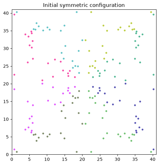
Visualize the Initial Configuration

plt.figure(figsize=(6, 6))
plt.scatter(positions[:, 0], positions[:, 1], c=colors, s=10, alpha=0.7)
plt.xlim(0, box)
plt.ylim(0, box)
plt.gca().set_aspect('equal')
plt.title('Initial symmetric configuration')
plt.show()

FIRE Minimization

Set up the periodic space and Lennard-Jones potential, then run FIRE to relax overlapping particles.

displacement, shift = space.periodic(box)
neighbor_fn, energy_fn = energy.lennard_jones_neighbor_list(displacement, box)

init_fn, step_fn = minimize.fire_descent(
  energy_fn, shift, dt_start=1e-7, dt_max=4e-7
)
step_fn = jit(step_fn)


@jit
def minimize_step(state, nbrs):
  state = step_fn(state, neighbor=nbrs)
  nbrs = nbrs.update(state.position)
  return state, nbrs


nbrs = neighbor_fn.allocate(positions, extra_capacity=6)
state = init_fn(positions, neighbor=nbrs)

min_steps = 100
for i in range(min_steps):
  state, nbrs = minimize_step(state, nbrs)
print(f'Minimization done. Neighborlist overflow: {nbrs.did_buffer_overflow}')

Minimization done. Neighborlist overflow: 0

NVT Simulation with Symmetry Folding

Define a helper that re-folds particles into their symmetric images after each integration step.

def fold_particles(group, box, n):
  def fold_fn(state):
    R = state.position
    V = state.momentum / state.mass
    R = R / box - 0.5
    R_homo = jnp.concatenate((R[:n], jnp.ones((n, 1))), axis=-1)
    V_homo = jnp.concatenate((V[:n], jnp.zeros((n, 1))), axis=-1)
    for i, s in enumerate(group.genpos):
      g = symd.str2mat(s)
      R = R.at[i * n:(i + 1) * n].set(jnp.fmod(R_homo @ g, 1.0)[:, :2])
      V = V.at[i * n:(i + 1) * n].set((V_homo @ g)[:, :2])
    R = box * (R + 0.5)
    return dataclasses.replace(state, position=R, momentum=V * state.mass)
  return fold_fn


fold_fn = fold_particles(group, box, N)

init_fn, step_fn = simulate.nvt_nose_hoover(
  energy_fn, shift, dt=1e-3, kT=0.8
)
step_fn = jit(step_fn)

state = init_fn(key, state.position, neighbor=nbrs)
state = dataclasses.replace(state, momentum=velocities * state.mass)

Run the NVT simulation, recording the trajectory.

def sim_fn(i, state_nbrs):
  state, nbrs = state_nbrs
  state = step_fn(state, neighbor=nbrs)
  state = fold_fn(state)
  nbrs = nbrs.update(state.position)
  return state, nbrs


n_records = 50 if SMOKE_TEST else 200
inner_steps = 10 if SMOKE_TEST else 100

trajectory = []
for i in range(n_records):
  trajectory += [state.position]
  state, nbrs = lax.fori_loop(0, inner_steps, sim_fn, (state, nbrs))
trajectory = jnp.stack(trajectory)
print(f'Simulation done. Neighborlist overflow: {nbrs.did_buffer_overflow}')

Simulation done. Neighborlist overflow: 0

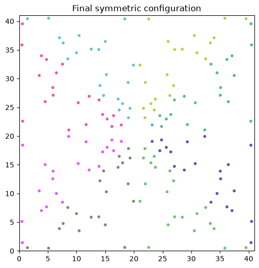
Visualize the Final Configuration

plt.figure(figsize=(6, 6))
plt.scatter(
  trajectory[-1][:, 0], trajectory[-1][:, 1],
  c=colors, s=10, alpha=0.7,
)
plt.xlim(0, box)
plt.ylim(0, box)
plt.gca().set_aspect('equal')
plt.title('Final symmetric configuration')
plt.show()

Trajectory Animation

from matplotlib.animation import FuncAnimation, PillowWriter
from IPython.display import Image, display

fig, ax = plt.subplots(figsize=(6, 6))

n_frames = len(trajectory)
stride = max(1, n_frames // 40)
frames = range(0, n_frames, stride)


def update(frame):
  ax.clear()
  ax.scatter(
    trajectory[frame][:, 0], trajectory[frame][:, 1],
    c=colors, s=10, alpha=0.7,
  )
  ax.set_xlim(0, float(box))
  ax.set_ylim(0, float(box))
  ax.set_aspect('equal')
  ax.set_title(f'Step {frame * inner_steps}')


anim = FuncAnimation(fig, update, frames=frames, interval=80)
anim.save('symd_trajectory.gif', writer=PillowWriter(fps=12))
plt.close(fig)
display(Image(filename='symd_trajectory.gif'))

<IPython.core.display.Image object>