Microcanonical Ensemble (NVE)

Here we demonstrate some code to run a simulation at constant energy. We start off by setting up some parameters of the simulation.

Imports & Utils

import os

IN_COLAB = 'COLAB_RELEASE_TAG' in os.environ
if IN_COLAB:
  import subprocess
  import sys

  subprocess.run(
    [
      sys.executable,
      '-m',
      'pip',
      'install',
      '-q',
      'git+https://github.com/jax-md/jax-md.git',
    ]
  )

import numpy as onp

from jax import config

config.update('jax_enable_x64', True)
import jax.numpy as np
from jax import random
from jax import jit
from jax import lax

import time
import os
from jax_md import space, smap, energy, minimize, quantity, simulate

import matplotlib
import matplotlib.pyplot as plt
import seaborn as sns

SMOKE_TEST = os.environ.get('READTHEDOCS', False)

sns.set_style(style='white')


def format_plot(x, y):
  plt.xlabel(x, fontsize=20)
  plt.ylabel(y, fontsize=20)


def finalize_plot(shape=(1, 1)):
  plt.gcf().set_size_inches(
    shape[0] * 1.5 * plt.gcf().get_size_inches()[1],
    shape[1] * 1.5 * plt.gcf().get_size_inches()[1],
  )
  plt.tight_layout()

Setup Simulation Parameters

N = 500 if SMOKE_TEST else 5000
dimension = 2
box_size = 40.0 if SMOKE_TEST else 80.0
displacement, shift = space.periodic(box_size)

Generate Random Positions and Particle Sizes

Next we need to generate some random positions as well as particle sizes.

key = random.PRNGKey(0)

R = random.uniform(
  key, (N, dimension), minval=0.0, maxval=box_size, dtype=np.float64
)

# The system ought to be a 50:50 mixture of two types of particles, one
# large and one small.
sigma = np.array([[1.0, 1.2], [1.2, 1.4]])
N_2 = int(N / 2)
species = np.where(np.arange(N) < N_2, 0, 1)

Construct Simulation Operators

Then we need to construct our simulation operators.

energy_fn = energy.soft_sphere_pair(displacement, species=species, sigma=sigma)
init, apply = simulate.nve(energy_fn, shift, 1e-2)
step = jit(lambda i, state: apply(state))
state = init(key, R, kT=0.0)

Run the Simulation

Now let’s actually do the simulation. We’ll keep track of potential energy and kinetic energy as the simulation progresses.

PE = []
KE = []
N_steps = 200 if SMOKE_TEST else 2000
print_every = 20
old_time = time.time()
print('Step\tKE\tPE\tTotal Energy\ttime/step')
print('----------------------------------------')

for i in range(N_steps):
  state = lax.fori_loop(0, 10, step, state)

  PE += [energy_fn(state.position)]
  KE += [quantity.kinetic_energy(momentum=state.momentum)]

  if i % print_every == 0 and i > 0:
    new_time = time.time()
    print(
      '{}\t{:.2f}\t{:.2f}\t{:.3f}\t{:.2f}'.format(
        i * print_every,
        KE[-1],
        PE[-1],
        KE[-1] + PE[-1],
        (new_time - old_time) / print_every / 10.0,
      )
    )
    old_time = new_time

PE = np.array(PE)
KE = np.array(KE)
R = state.position

Step    KE      PE      Total Energy    time/step
----------------------------------------
400     26.30   5.45    31.759  0.03
800     26.99   4.77    31.759  0.02
1200    26.81   4.95    31.759  0.02
1600    26.78   4.98    31.759  0.02
2000    25.42   6.33    31.759  0.02
2400    27.39   4.36    31.759  0.02
2800    25.59   6.17    31.759  0.02
3200    25.91   5.85    31.759  0.02
3600    26.25   5.51    31.759  0.02

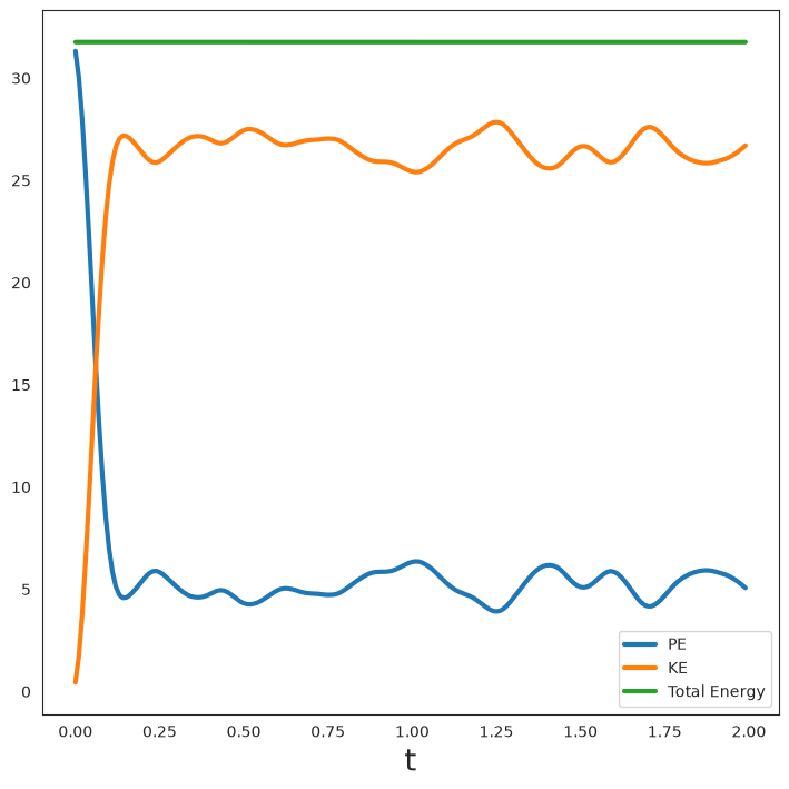
Plot Energy Evolution

Now, let’s plot the energy as a function of time. We see that the initial potential energy goes down, the kinetic energy goes up, but the total energy stays constant.

t = onp.arange(0, N_steps) * 1e-2
plt.plot(t, PE, label='PE', linewidth=3)
plt.plot(t, KE, label='KE', linewidth=3)
plt.plot(t, PE + KE, label='Total Energy', linewidth=3)
plt.legend()
format_plot('t', '')
finalize_plot()

Visualize the System

Now let’s plot the system.

ms = 40 if SMOKE_TEST else 20
R_plt = onp.array(state.position)

plt.plot(R_plt[:N_2, 0], R_plt[:N_2, 1], 'o', markersize=ms * 0.5)
plt.plot(R_plt[N_2:, 0], R_plt[N_2:, 1], 'o', markersize=ms * 0.7)

plt.xlim([0, np.max(R[:, 0])])
plt.ylim([0, np.max(R[:, 1])])

plt.axis('off')

finalize_plot((2, 2))