Canonical Ensemble (NVT) - Nose-Hoover#
Here we demonstrate some code to run a simulation at in the NVT ensemble. We start off by setting up some parameters of the simulation. This will include a temperature schedule that will start off at a high temperature and then instantaneously quench to a lower temperature.
Imports & Utils#
[1]:
import os

IN_COLAB = 'COLAB_RELEASE_TAG' in os.environ
if IN_COLAB:
  import subprocess
  import sys

  subprocess.run(
    [
      sys.executable,
      '-m',
      'pip',
      'install',
      '-q',
      'git+https://github.com/jax-md/jax-md.git',
    ]
  )

import numpy as onp

from jax import config

config.update('jax_enable_x64', True)
import jax.numpy as np
from jax import random
from jax import jit
from jax import lax
from jax import ops

import time

from jax_md import space, smap, energy, minimize, quantity, simulate

import matplotlib
import matplotlib.pyplot as plt
import seaborn as sns

SMOKE_TEST = os.environ.get('READTHEDOCS', False)

sns.set_style(style='white')


def format_plot(x, y):
  plt.xlabel(x, fontsize=20)
  plt.ylabel(y, fontsize=20)


def finalize_plot(shape=(1, 1)):
  plt.gcf().set_size_inches(
    shape[0] * 1.5 * plt.gcf().get_size_inches()[1],
    shape[1] * 1.5 * plt.gcf().get_size_inches()[1],
  )
  plt.tight_layout()
Setup Simulation Parameters#
[2]:
N = 500
dimension = 2
box_size = quantity.box_size_at_number_density(N, 0.8, 2)
dt = 5e-3
displacement, shift = space.periodic(box_size)

steps = 4000 if SMOKE_TEST else 10000
max_time = steps * dt
kT = lambda t: np.where(t < max_time / 2, 0.1, 0.01)
Generate Random Positions and Particle Sizes#
Next we need to generate some random positions as well as particle sizes.
[3]:
key = random.PRNGKey(0)
[4]:
key, split = random.split(key)
R = box_size * random.uniform(split, (N, dimension), dtype=np.float64)

# The system ought to be a 50:50 mixture of two types of particles, one
# large and one small.
sigma = np.array([[1.0, 1.2], [1.2, 1.4]])
N_2 = int(N / 2)
species = np.where(np.arange(N) < N_2, 0, 1)
Construct Simulation Operators#
Then we need to construct our simulation operators.
[5]:
energy_fn = energy.soft_sphere_pair(displacement, species=species, sigma=sigma)

init, apply = simulate.nvt_nose_hoover(energy_fn, shift, dt, kT(0.0))
state = init(key, R)
Define Step Function with Logging#
Now let’s actually do the simulation. To do this we’ll write a small function that performs a single step of the simulation. This function will keep track of the temperature, the extended Hamiltonian of the Nose-Hoover dynamics, and the current particle positions.
[6]:
write_every = 100


def step_fn(i, state_and_log):
  state, log = state_and_log

  t = i * dt

  # Log information about the simulation.
  T = quantity.temperature(momentum=state.momentum)
  log['kT'] = log['kT'].at[i].set(T)
  H = simulate.nvt_nose_hoover_invariant(energy_fn, state, kT(t))
  log['H'] = log['H'].at[i].set(H)
  # Record positions every `write_every` steps.
  log['position'] = lax.cond(
    i % write_every == 0,
    lambda p: p.at[i // write_every].set(state.position),
    lambda p: p,
    log['position'],
  )

  # Take a simulation step.
  state = apply(state, kT=kT(t))

  return state, log
Run the Simulation#
To run our simulation we’ll use lax.fori_loop which will execute the simulation a single call from python.
[7]:
log = {
  'kT': np.zeros((steps,)),
  'H': np.zeros((steps,)),
  'position': np.zeros((steps // write_every,) + R.shape),
}

state, log = lax.fori_loop(0, steps, step_fn, (state, log))

R = state.position
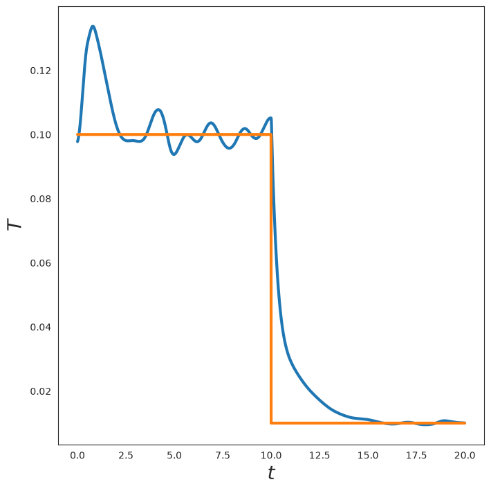
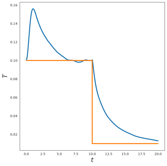
Plot Temperature Evolution#
Now, let’s plot the temperature as a function of time. We see that the temperature tracks the goal temperature with some fluctuations.
[8]:
t = onp.arange(0, steps) * dt
plt.plot(t, log['kT'], linewidth=3)
plt.plot(t, kT(t), linewidth=3)
format_plot('$t$', '$T$')
finalize_plot()
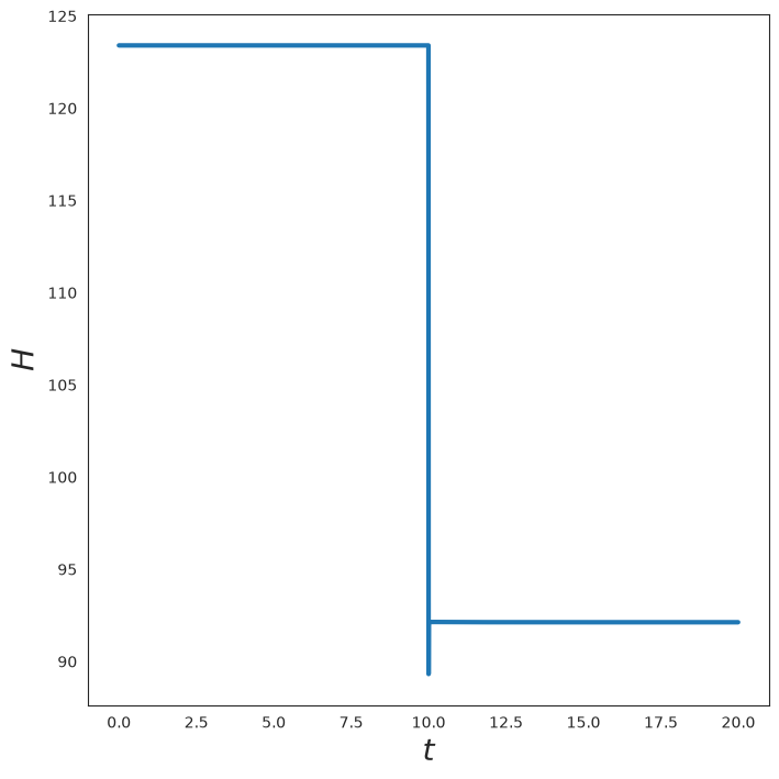
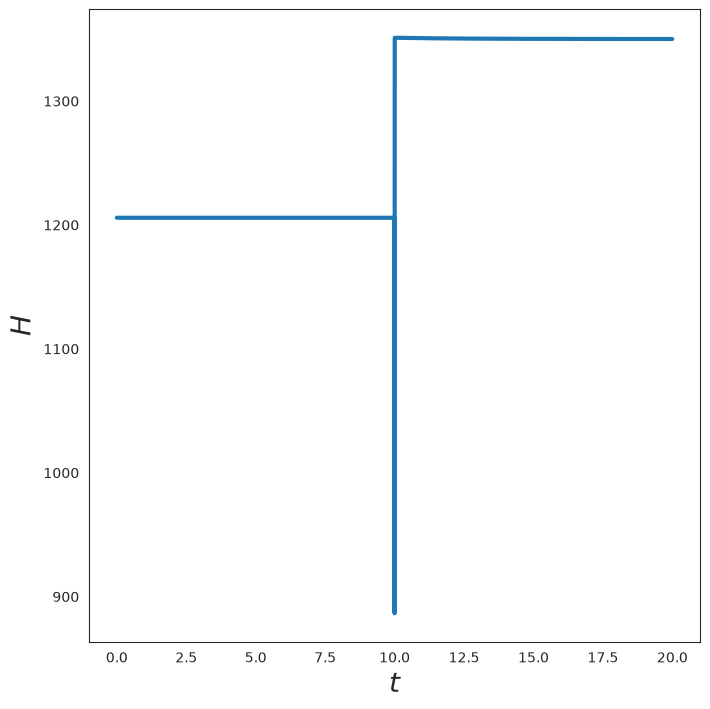
Plot NVT Hamiltonian#
Now let’s plot the Hamiltonian of the system. We see that it is invariant apart from changes to the temperature, as expected.
[9]:
plt.plot(t, log['H'], linewidth=3)
format_plot('$t$', '$H$')
finalize_plot()
Visualize the System#
Now let’s plot a snapshot of the system.
[10]:
ms = 65
R_plt = onp.array(state.position)

plt.plot(R_plt[:N_2, 0], R_plt[:N_2, 1], 'o', markersize=ms * 0.5)
plt.plot(R_plt[N_2:, 0], R_plt[N_2:, 1], 'o', markersize=ms * 0.7)

plt.xlim([0, np.max(R[:, 0])])
plt.ylim([0, np.max(R[:, 1])])

plt.axis('off')

finalize_plot((2, 2))

Animation (Optional)#
If we want, we can also draw an animation of the simulation using JAX MD’s renderer. This only works in Google Colab.
[11]:
if IN_COLAB:
  from jax_md.colab_tools import renderer

  diameters = sigma[species, species]
  colors = np.where(
    species[:, None],
    np.array([[1.0, 0.5, 0.01]]),
    np.array([[0.35, 0.65, 0.85]]),
  )

  renderer.render(
    box_size,
    {'particles': renderer.Disk(log['position'], diameters, colors)},
    resolution=(700, 700),
  )
else:
  print('Renderer only available in Google Colab. Skipping.')
Renderer only available in Google Colab. Skipping.
Larger Simulation with Neighbor Lists#
We can use neighbor lists to run a much larger version of this simulation. As their name suggests, neighbor lists are lists of particles nearby a central particle. By keeping track of neighbors, we can compute the energy of the system much more efficiently. This becomes increasingly true as the simulation gets larger.
[12]:
N = 4800 if SMOKE_TEST else 128000
box_size = quantity.box_size_at_number_density(N, 0.8, 2)
displacement, shift = space.periodic(box_size)
Initialize Large System#
As before we randomly initialize the system.
[13]:
key, split = random.split(key)
R = box_size * random.uniform(split, (N, dimension), dtype=np.float64)

sigma = np.array([[1.0, 1.2], [1.2, 1.4]])
N_2 = int(N / 2)
species = np.where(np.arange(N) < N_2, 0, 1)
Construct Neighbor List and Energy Function#
Then we need to construct our simulation operators. This time we use the energy.soft_sphere_neighbor_fn to create two functions: one that constructs lists of neighbors and one that computes the energy.
[14]:
neighbor_fn, energy_fn = energy.soft_sphere_neighbor_list(
  displacement, box_size, species=species, sigma=sigma
)

init, apply = simulate.nvt_nose_hoover(
  energy_fn, shift, dt, kT(0.0), tau=200 * dt
)

nbrs = neighbor_fn.allocate(R)
state = init(key, R, neighbor=nbrs)
Run Large Simulation#
Now let’s actually do the simulation. This time our simulation step function will also update the neighbors. As above, we will also only record position data every hundred steps.
[15]:
write_every = 100


def step_fn(i, state_nbrs_log):
  state, nbrs, log = state_nbrs_log

  t = i * dt

  # Log information about the simulation.
  T = quantity.temperature(momentum=state.momentum)
  log['kT'] = log['kT'].at[i].set(T)
  H = simulate.nvt_nose_hoover_invariant(energy_fn, state, kT(t), neighbor=nbrs)
  log['H'] = log['H'].at[i].set(H)
  # Record positions every `write_every` steps.
  log['position'] = lax.cond(
    i % write_every == 0,
    lambda p: p.at[i // write_every].set(state.position),
    lambda p: p,
    log['position'],
  )

  # Take a simulation step.
  state = apply(state, kT=kT(t), neighbor=nbrs)
  nbrs = nbrs.update(state.position)

  return state, nbrs, log
To run our simulation we’ll use lax.fori_loop which will execute the simulation a single call from python.
[16]:
steps = 4000 if SMOKE_TEST else 20000
max_time = steps * dt
kT = lambda t: np.where(t < max_time / 2, 0.1, 0.01)

log = {
  'kT': np.zeros((steps,)),
  'H': np.zeros((steps,)),
  'position': np.zeros((steps // write_every,) + R.shape),
}

state, nbrs, log = lax.fori_loop(0, steps, step_fn, (state, nbrs, log))

R = state.position
Plot Results for Large Simulation#
Now, let’s plot the temperature as a function of time. We see that the temperature tracks the goal temperature with some fluctuations.
[17]:
t = onp.arange(0, steps) * dt
plt.plot(t, log['kT'], linewidth=3)
plt.plot(t, kT(t), linewidth=3)
format_plot('$t$', '$T$')
finalize_plot()
Now let’s plot the Hamiltonian of the system. We see that it is invariant apart from changes to the temperature, as expected.
[18]:
plt.plot(t, log['H'], linewidth=3)
format_plot('$t$', '$H$')
finalize_plot()
Visualize Large System#
Now let’s plot a snapshot of the system.
[19]:
ms = 10 if SMOKE_TEST else 1
R_plt = onp.array(state.position)

plt.plot(R_plt[:N_2, 0], R_plt[:N_2, 1], 'o', markersize=ms * 0.5)
plt.plot(R_plt[N_2:, 0], R_plt[N_2:, 1], 'o', markersize=ms * 0.7)

plt.xlim([0, np.max(R[:, 0])])
plt.ylim([0, np.max(R[:, 1])])

plt.axis('off')

finalize_plot((2, 2))

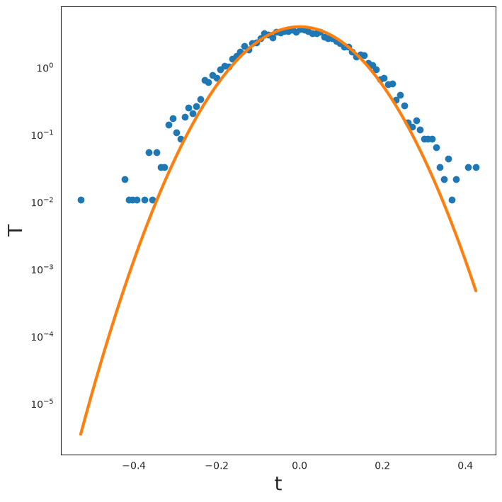
Velocity Distribution#
Finally, let’s plot the velocity distribution compared with its theoretical prediction.
[20]:
V_flat = onp.reshape(onp.array(state.velocity), (-1,))
occ, bins = onp.histogram(V_flat, bins=100, density=True)
[21]:
T_cur = kT(steps * dt)
plt.semilogy(bins[:-1], occ, 'o')
plt.semilogy(
  bins[:-1],
  1.0 / np.sqrt(2 * np.pi * T_cur) * onp.exp(-1 / (2 * T_cur) * bins[:-1] ** 2),
  linewidth=3,
)
format_plot('t', 'T')
finalize_plot()