Harmonic Minimization

Here we demonstrate some simple example code showing how we might find the inherent structure for some initially random configuration of particles. Note that this code will work on CPU, GPU, or TPU out of the box.

First thing we need to do is set some parameters that define our simulation, including what kind of box we’re using (specified using a metric function and a wrapping function).

Imports & Utils

import os

IN_COLAB = 'COLAB_RELEASE_TAG' in os.environ
if IN_COLAB:
  import subprocess
  import sys

  subprocess.run(
    [
      sys.executable,
      '-m',
      'pip',
      'install',
      '-q',
      'git+https://github.com/jax-md/jax-md.git',
    ]
  )

import numpy as onp

import jax.numpy as np
from jax import config

config.update('jax_enable_x64', True)

from jax import random
from jax import jit

from jax_md import space, smap, energy, minimize, quantity, simulate

import matplotlib
import matplotlib.pyplot as plt
import seaborn as sns

sns.set_style(style='white')


def format_plot(x, y):
  plt.grid(True)
  plt.xlabel(x, fontsize=20)
  plt.ylabel(y, fontsize=20)


def finalize_plot(shape=(1, 1)):
  plt.gcf().set_size_inches(
    shape[0] * 1.5 * plt.gcf().get_size_inches()[1],
    shape[1] * 1.5 * plt.gcf().get_size_inches()[1],
  )
  plt.tight_layout()


# Check if running in ReadTheDocs environment
SMOKE_TEST = os.environ.get('READTHEDOCS', False)

System Setup

# Simulation parameters
N = 400 if SMOKE_TEST else 1000
dimension = 2
box_size = quantity.box_size_at_number_density(N, 0.8, dimension)
displacement, shift = space.periodic(box_size)

Next we need to generate some random positions as well as particle sizes.

key = random.PRNGKey(0)

R = box_size * random.uniform(key, (N, dimension), dtype=np.float32)

# The system ought to be a 50:50 mixture of two types of particles, one
# large and one small.
sigma = np.array([[1.0, 1.2], [1.2, 1.4]])
N_2 = int(N / 2)
species = np.where(np.arange(N) < N_2, 0, 1)

FIRE Minimization

Then we need to construct our FIRE minimization function. Like all simulations in JAX MD, the FIRE optimizer is two functions: an init_fn that creates the state of the optimizer and an apply_fn that updates the state to a new state.

energy_fn = energy.soft_sphere_pair(displacement, species=species, sigma=sigma)
fire_init, fire_apply = minimize.fire_descent(energy_fn, shift)
fire_apply = jit(fire_apply)
fire_state = fire_init(R)

Now let’s actually do minimization, keeping track of the energy and particle positions as we go.

E = []
trajectory = []

# Use fewer iterations for SMOKE_TEST
max_steps = 200

for i in range(max_steps):
  fire_state = fire_apply(fire_state)

  E += [energy_fn(fire_state.position)]
  trajectory += [fire_state.position]

R = fire_state.position
trajectory = np.stack(trajectory)

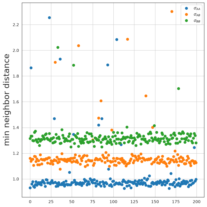
Analysis

Let’s plot the nearest distance for different species pairs. We see that particles on average have neighbors that are the right distance apart.

metric = lambda R: space.distance(space.map_product(displacement)(R, R))
dr = metric(R)
plt.plot(
  np.min(dr[:N_2, :N_2] + 5 * np.eye(N_2, N_2), axis=0),
  'o',
  label='$\\sigma_{AA}$',
)
plt.plot(
  np.min(dr[:N_2, N_2:] + 5 * np.eye(N_2, N_2), axis=0),
  'o',
  label='$\\sigma_{AB}$',
)
plt.plot(
  np.min(dr[N_2:, N_2:] + 5 * np.eye(N_2, N_2), axis=0),
  'o',
  label='$\\sigma_{BB}$',
)

plt.legend()
format_plot('', 'min neighbor distance')
finalize_plot()

Now let’s plot the system. It’s nice and minimized!

ms = 45
R_plt = onp.array(fire_state.position)

plt.plot(R_plt[:N_2, 0], R_plt[:N_2, 1], 'o', markersize=ms * 0.5)
plt.plot(R_plt[N_2:, 0], R_plt[N_2:, 1], 'o', markersize=ms * 0.7)

plt.xlim([0, np.max(R[:, 0])])
plt.ylim([0, np.max(R[:, 1])])

plt.axis('off')

finalize_plot((2, 2))

If we want, we can visualize the entire minimization.

if IN_COLAB:
  from jax_md.colab_tools import renderer

  diameter = np.where(species, 1.4, 1.0)
  color = np.where(
    species[:, None],
    np.array([[1.0, 0.5, 0.05]]),
    np.array([[0.15, 0.45, 0.8]]),
  )
  renderer.render(
    box_size,
    {'particles': renderer.Disk(trajectory, diameter, color)},
    buffer_size=50,
  )

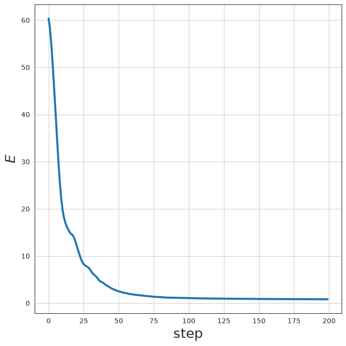
Finally, let’s plot the energy trajectory that we observed during FIRE minimization.

plt.plot(E, linewidth=3)

format_plot('step', '$E$')
finalize_plot()