Microcanonical Ensemble (NVE) with Neighbor Lists

Imports & Utils

import os

IN_COLAB = 'COLAB_RELEASE_TAG' in os.environ
if IN_COLAB:
  import subprocess
  import sys

  subprocess.run(
    [
      sys.executable,
      '-m',
      'pip',
      'install',
      '-q',
      'git+https://github.com/jax-md/jax-md.git',
    ]
  )

import numpy as onp

from jax import config

config.update('jax_enable_x64', True)
import jax.numpy as np
from jax import random
from jax import jit
from jax import lax

import time
import os
from jax_md import space
from jax_md import smap
from jax_md import energy
from jax_md import quantity
from jax_md import simulate
from jax_md import partition

import matplotlib
import matplotlib.pyplot as plt
import seaborn as sns

sns.set_style(style='white')

SMOKE_TEST = os.environ.get('READTHEDOCS', False)


def format_plot(x, y):
  plt.xlabel(x, fontsize=20)
  plt.ylabel(y, fontsize=20)


def finalize_plot(shape=(1, 1)):
  plt.gcf().set_size_inches(
    shape[0] * 1.5 * plt.gcf().get_size_inches()[1],
    shape[1] * 1.5 * plt.gcf().get_size_inches()[1],
  )
  plt.tight_layout()

Setup System Parameters

Nx = particles_per_side = 30 if SMOKE_TEST else 80
spacing = np.float32(1.25)
side_length = Nx * spacing

R = onp.stack([onp.array(r) for r in onp.ndindex(Nx, Nx)]) * spacing
R = np.array(R, np.float64)

Draw the Initial State

ms = 40 if SMOKE_TEST else 16
R_plt = onp.array(R)

plt.plot(R_plt[:, 0], R_plt[:, 1], 'o', markersize=ms * 0.5)

plt.xlim([0, np.max(R[:, 0])])
plt.ylim([0, np.max(R[:, 1])])

plt.axis('off')

finalize_plot((2, 2))

Neighbor List Formats

JAX MD supports three different formats for neighbor lists: Dense, Sparse, and OrderedSparse.

Dense neighbor lists store neighbor IDs in a matrix of shape (particle_count, neighbors_per_particle). This can be advantageous if the system if homogeneous since it requires less memory bandwidth. However, Dense neighbor lists are more prone to overflows or waste if there are large fluctuations in the number of neighbors, since they must allocate enough capacity for the maximum number of neighbors.

Sparse neighbor lists store neighbor IDs in a matrix of shape (2, total_neighbors) where the first index specifies senders and receivers for each neighboring pair. Unlike Dense neighbor lists, Sparse neighbor lists must store two integers for each neighboring pair. However, they benefit because their capacity is bounded by the total number of neighbors, making them more efficient when different particles have different numbers of neighbors.

OrderedSparse neighbor lists are like Sparse neighbor lists, except they only store pairs of neighbors (i, j) where i < j. For potentials that can be phrased as \(\sum_{i<j}E_{ij}\) this can give a factor of two improvement in speed.

# format = partition.Dense
# format = partition.Sparse
format = partition.OrderedSparse

Construct Energy Functions

Construct two versions of the energy function with and without neighbor lists.

displacement, shift = space.periodic(side_length)

neighbor_fn, energy_fn = energy.lennard_jones_neighbor_list(
  displacement, side_length, format=format
)
energy_fn = jit(energy_fn)

exact_energy_fn = jit(energy.lennard_jones_pair(displacement))

Allocate Neighbor List

To use a neighbor list, we must first allocate it. This step cannot be Just-in-Time (JIT) compiled because it uses the state of the system to infer the capacity of the neighbor list (which involves dynamic shapes).

nbrs = neighbor_fn.allocate(R)

Compare Energy Calculations

Now we can compute the energy with and without neighbor lists. We see that both results agree, but the neighbor list version of the code is significantly faster.

# Run once so that we avoid the jit compilation time.
print('E = {}'.format(energy_fn(R, neighbor=nbrs)))
print('E_ex = {}'.format(exact_energy_fn(R)))

E = -1620.855226368001
E_ex = -1620.8552263679999

Benchmark neighbor list version:

energy_fn(R, neighbor=nbrs).block_until_ready()

Array(-1620.85522637, dtype=float64)

Benchmark exact version (without neighbor lists):

exact_energy_fn(R).block_until_ready()

Array(-1620.85522637, dtype=float64)

Run Simulation with Neighbor Lists

Now we can run a simulation. Inside the body of the simulation, we update the neighbor list using nbrs.update(position). This can be JIT, but it also might lead to buffer overflows if the allocated neighborlist cannot accomodate all of the neighbors. Therefore, every so often we check whether the neighbor list overflowed and if it did, we reallocate it using the state right before it overflowed.

displacement, shift = space.periodic(side_length)

init_fn, apply_fn = simulate.nve(energy_fn, shift, 1e-3)
state = init_fn(random.PRNGKey(0), R, kT=1e-3, neighbor=nbrs)


def body_fn(i, state):
  state, nbrs = state
  nbrs = nbrs.update(state.position)
  state = apply_fn(state, neighbor=nbrs)
  return state, nbrs


step = 0
while step < (20 if SMOKE_TEST else 40):
  new_state, nbrs = lax.fori_loop(0, 100, body_fn, (state, nbrs))
  if nbrs.did_buffer_overflow:
    print('Neighbor list overflowed, reallocating.')
    nbrs = neighbor_fn.allocate(state.position)
  else:
    state = new_state
    step += 1

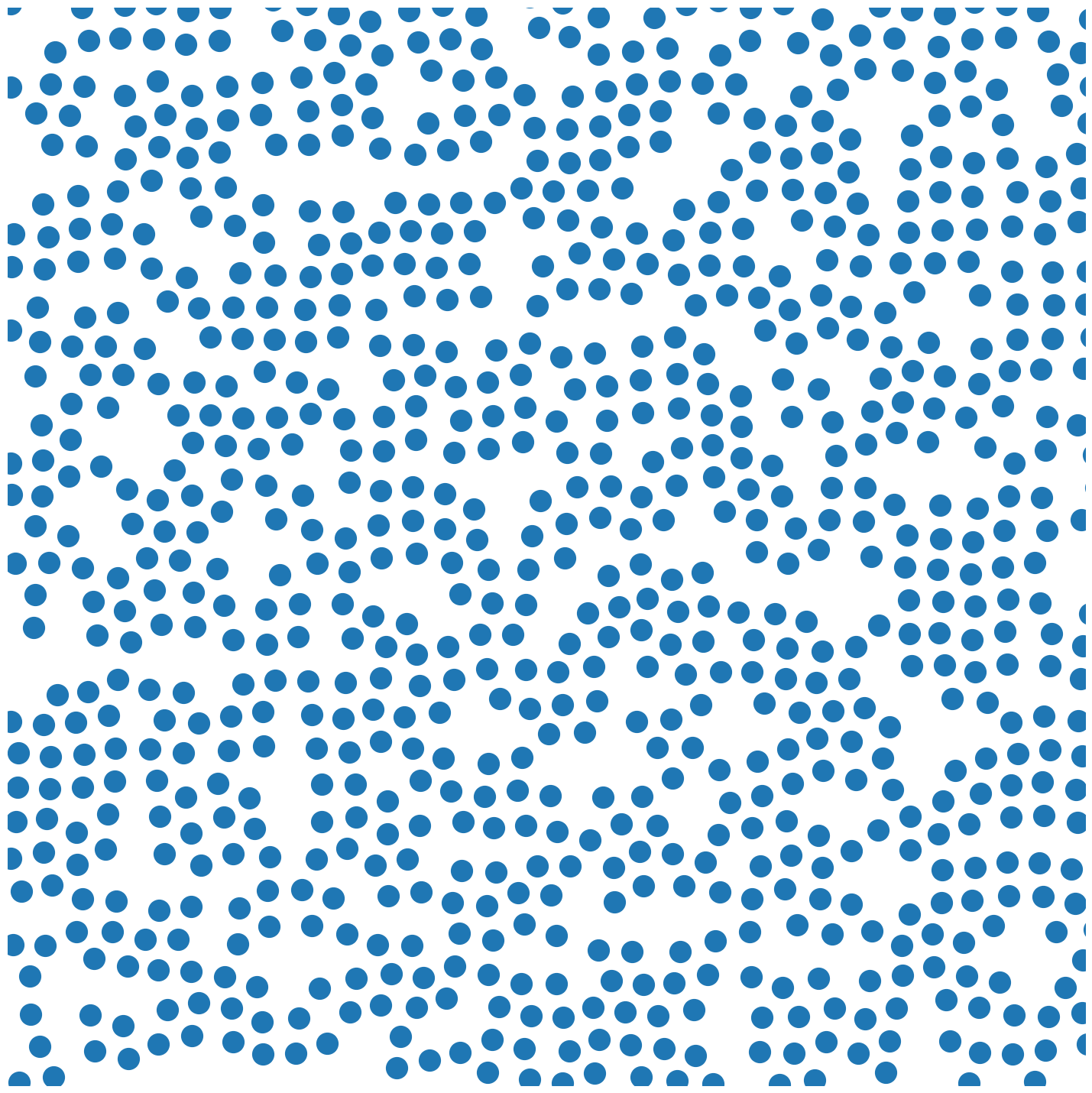
Draw the Final State

ms = 40 if SMOKE_TEST else 16
R_plt = onp.array(state.position)

plt.plot(R_plt[:, 0], R_plt[:, 1], 'o', markersize=ms * 0.5)

plt.xlim([0, np.max(R[:, 0])])
plt.ylim([0, np.max(R[:, 1])])

plt.axis('off')

finalize_plot((2, 2))