Isothermal-Isobaric Ensemble (NPT) - Nose-Hoover

Here we demonstrate some code to run a simulation at in the NPT ensemble with constant temperature and pressure. We start off by setting up some parameters of the simulation. This will include a pressure schedule that will start off at a relatively low pressure before instantaneously trippling the pressure.

Note that unlike in the case of NVT and NVE simulations, NPT simulations must be performed with periodic_general boundary conditions. For now NPT simulations must be performed with fractional coordinates, where the atom positions are stored in the unit cube. This restriction can likely be relaxed in the future, if it were desirable.

Imports & Utils

import os

IN_COLAB = 'COLAB_RELEASE_TAG' in os.environ
if IN_COLAB:
  import subprocess
  import sys

  subprocess.run(
    [
      sys.executable,
      '-m',
      'pip',
      'install',
      '-q',
      'git+https://github.com/jax-md/jax-md.git',
    ]
  )

import numpy as onp

from jax import config

config.update('jax_enable_x64', True)
import jax.numpy as np
from jax import random
from jax import jit
from jax import lax
from jax import ops

import time

from jax_md import space, smap, energy, minimize, quantity, simulate

import matplotlib
import matplotlib.pyplot as plt
import seaborn as sns

sns.set_style(style='white')

SMOKE_TEST = os.environ.get('READTHEDOCS', False)


def format_plot(x, y):
  plt.xlabel(x, fontsize=20)
  plt.ylabel(y, fontsize=20)


def finalize_plot(shape=(1, 1)):
  plt.gcf().set_size_inches(
    shape[0] * 1.5 * plt.gcf().get_size_inches()[1],
    shape[1] * 1.5 * plt.gcf().get_size_inches()[1],
  )
  plt.tight_layout()

Setup Simulation Parameters

N = 200 if SMOKE_TEST else 400
dimension = 2
box = quantity.box_size_at_number_density(N, 0.8, 2)
dt = 5e-3
displacement, shift = space.periodic_general(box)

steps = 4000 if SMOKE_TEST else 40000
max_time = steps * dt
kT = np.float32(0.01)
P = lambda t: np.where(t < max_time / 2, 0.05, 0.15)

Generate Random Positions and Particle Sizes

Next we need to generate some random positions as well as particle sizes. Because we are using periodic_general boundary conditions with fractional coordinates, we produce initial particle positions in the unit cube.

key = random.PRNGKey(0)

key, split = random.split(key)
R = random.uniform(split, (N, dimension), dtype=np.float64)

# The system ought to be a 50:50 mixture of two types of particles, one
# large and one small.
sigma = np.array([[1.0, 1.2], [1.2, 1.4]])
N_2 = int(N / 2)
species = np.where(np.arange(N) < N_2, 0, 1)

Construct Simulation Operators

Then we need to construct our simulation operators.

energy_fn = energy.soft_sphere_pair(displacement, species=species, sigma=sigma)

init, apply = simulate.npt_nose_hoover(energy_fn, shift, dt, P(0.0), kT)
state = init(key, R, box)

Define Step Function with Logging

Now let’s actually do the simulation. To do this we’ll write a small function that performs a single step of the simulation. This function will keep track of the temperature, the extended Hamiltonian of the Nose-Hoover dynamics, and the current particle positions.

write_every = 100


def step_fn(i, state_and_log):
  state, log = state_and_log

  t = i * dt

  # Log information about the simulation.
  T = quantity.temperature(momentum=state.momentum)
  log['kT'] = log['kT'].at[i].set(T)

  box = simulate.npt_box(state)
  KE = quantity.kinetic_energy(momentum=state.momentum)
  P_measured = quantity.pressure(energy_fn, state.position, box, KE)
  log['P'] = log['P'].at[i].set(P_measured)

  H = simulate.npt_nose_hoover_invariant(energy_fn, state, P(t), kT)
  log['H'] = log['H'].at[i].set(H)

  # Record positions every `write_every` steps.
  pos = space.transform(box, state.position)
  log['position'] = np.where(
    i % write_every == 0,
    log['position'].at[i // write_every].set(pos),
    log['position'],
  )

  # Take a simulation step.
  state = apply(state, pressure=P(t))

  return state, log

Run the Simulation

To run our simulation we’ll use lax.fori_loop which will execute the simulation a single call from python.

log = {
  'kT': np.zeros((steps,)),
  'P': np.zeros((steps,)),
  'H': np.zeros((steps,)),
  'position': np.zeros((steps // write_every,) + R.shape),
}

state, log = lax.fori_loop(0, steps, step_fn, (state, log))

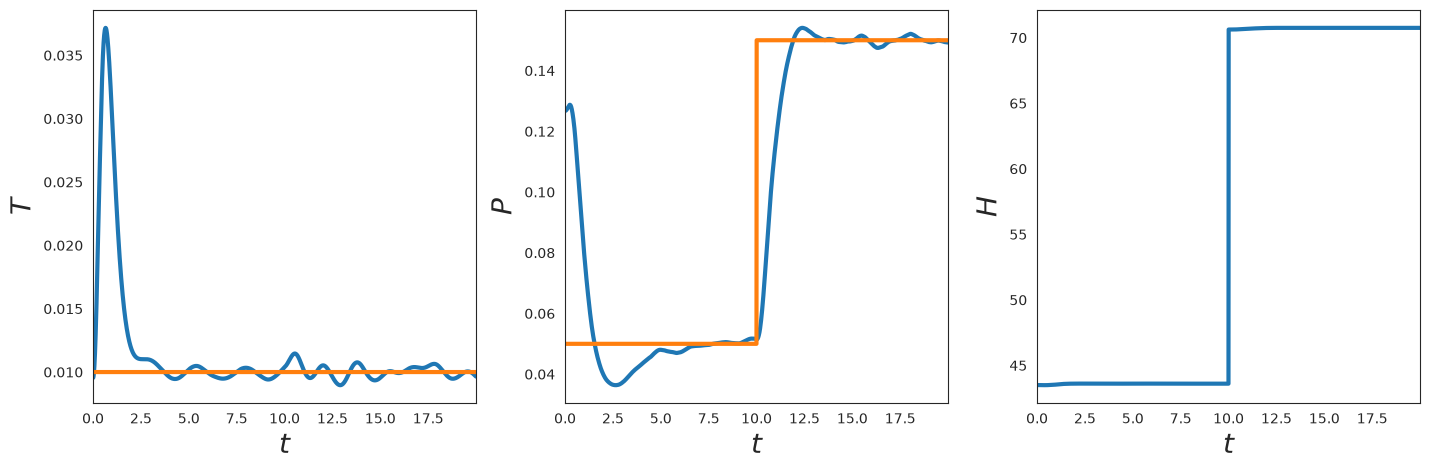
Plot Results

Now, let’s plot the temperature, pressure, and hamiltonian as a function of time. We see that the temperature and pressure track the target with some fluctuations. The Hamiltonian is exactly invariant apart from the point where the target pressure is changed discontinuously.

plt.subplot(1, 3, 1)

t = onp.arange(0, steps) * dt
plt.plot(t, log['kT'], linewidth=3)
plt.plot(t, kT * np.ones_like(t), linewidth=3)
plt.xlim([t[0], t[-1]])
format_plot('$t$', '$T$')

plt.subplot(1, 3, 2)

t = onp.arange(0, steps) * dt
plt.plot(t, log['P'], linewidth=3)
plt.plot(t, P(t), linewidth=3)
plt.xlim([t[0], t[-1]])
format_plot('$t$', '$P$')

plt.subplot(1, 3, 3)

t = onp.arange(0, steps) * dt
plt.plot(t, log['H'], linewidth=3)
plt.xlim([t[0], t[-1]])
format_plot('$t$', '$H$')

finalize_plot((2, 2 / 3))

Visualize the System

Now let’s plot a snapshot of the system.

ms = 65
R_plt = onp.array(log['position'][-1])

plt.plot(R_plt[:N_2, 0], R_plt[:N_2, 1], 'o', markersize=ms * 0.5)
plt.plot(R_plt[N_2:, 0], R_plt[N_2:, 1], 'o', markersize=ms * 0.7)

plt.xlim([0, np.max(R_plt[:, 0])])
plt.ylim([0, np.max(R_plt[:, 1])])

plt.axis('off')

finalize_plot((2, 2))

Animation (Optional)

If we want, we can also draw an animation of the simulation using JAX MD’s renderer. We see that the system starts out fluctuating about an initial larger box. When the pressure instantaneously changes, the box compresses the system. This only works in Google Colab.

if IN_COLAB:
  from jax_md.colab_tools import renderer

  diameters = sigma[species, species]
  colors = np.where(
    species[:, None],
    np.array([[1.0, 0.5, 0.01]]),
    np.array([[0.35, 0.65, 0.85]]),
  )

  renderer.render(
    box,
    {'particles': renderer.Disk(log['position'], diameters, colors)},
    resolution=(700, 700),
  )
else:
  print('Renderer only available in Google Colab. Skipping.')

Renderer only available in Google Colab. Skipping.

Larger Simulation with Neighbor Lists

Warning: This section is a work in progress. We hope to make NPT + neighbor lists more ergonimic and safe in the future.

We can use neighbor lists to run a much larger version of this simulation. As their name suggests, neighbor lists are lists of particles nearby a central particle. By keeping track of neighbors, we can compute the energy of the system much more efficiently. This becomes increasingly true as the simulation gets larger. Unlike other simulation environments, extra care must be taken with NPT simulations when using cell lists to construct neighbor lists (which is the default behavior). This is because the cells must be defined in the unit cube. As the system’s volume changes, the effective size of cells will change. At some point, this may invalidate cell list, either because of buffer overflows or because the cells become too small to cover the desired neighborhood size. While we have error checking in the former case, we do not yet have checks for the latter.

The code in this section therefore is to serve as an example for how neighbor lists + NPT might work. We expect to improve this section with time. If it is a priority for your work, please raise an issue.

As before, the first step here is to setup some simulation parameters. Unlike before, here we must be especially mindful of fluctuations in the box size. As such we will start out by creating the system and randomly initializing it. However, we will then minimize the system to its nearest minimum before starting the simulation.

N = 1000 if SMOKE_TEST else 10000
dt = 5e-3
box = quantity.box_size_at_number_density(N, 0.8, 2) * np.eye(2)
displacement, shift = space.periodic_general(box)

kT = np.float32(0.01)
max_time = steps * dt
P = lambda t: np.where(t < max_time / 2, 0.05, 0.07)

Initialize Large System

As before we randomly initialize the system.

key, split = random.split(key)
R = random.uniform(split, (N, dimension), dtype=np.float64)

sigma = np.array([[1.0, 1.2], [1.2, 1.4]])
N_2 = int(N / 2)
species = np.where(np.arange(N) < N_2, 0, 1)

Minimize System

Then we need to construct our simulation operators. This time we use the energy.soft_sphere_neighbor_fn to create two functions: one that constructs lists of neighbors and one that computes the energy. Since we store the particle positions fractionally (in the unit cube), we must pass fractional_coordinates=True to the energy function.

neighbor_fn, energy_fn = energy.soft_sphere_neighbor_list(
  displacement, box, species=species, sigma=sigma, fractional_coordinates=True
)

init, apply = minimize.fire_descent(energy_fn, shift)

nbrs = neighbor_fn.allocate(R, extra_capacity=5)

state = init(R, neighbor=nbrs)


def cond_fn(state_nbrs):
  state, nbrs = state_nbrs
  return np.any(np.abs(state.force) > 1e-3)


def step_fn(state_nbrs):
  state, nbrs = state_nbrs
  state = apply(state, neighbor=nbrs)
  nbrs = nbrs.update(state.position)
  return state, nbrs


state, nbrs = lax.while_loop(cond_fn, step_fn, (state, nbrs))

print(f'Did buffer overflow: {nbrs.did_buffer_overflow}')
print(
  f'Pressure: {quantity.pressure(energy_fn, state.position, box, neighbor=nbrs)}'
)

Did buffer overflow: 0
Pressure: 0.032011307079510526

Plot Minimized Configuration

Now we can plot the minimized configuration.

ms = 20 if SMOKE_TEST else 10
R_plt = onp.array(state.position)

plt.plot(R_plt[:N_2, 0], R_plt[:N_2, 1], 'o', markersize=ms * 0.5)
plt.plot(R_plt[N_2:, 0], R_plt[N_2:, 1], 'o', markersize=ms * 0.7)

plt.xlim([0, np.max(R[:, 0])])
plt.ylim([0, np.max(R[:, 1])])

plt.axis('off')

finalize_plot((2, 2))

Setup NPT Simulation with Neighbor Lists

Now that we have a minimized configuration, we can do an NPT simulation. Since our cells have a fixed size, the neighbor list that we constructed will become invalid if the box is too small.

init, apply = simulate.npt_nose_hoover(energy_fn, shift, dt, P(0.0), kT)

nbrs = neighbor_fn.allocate(state.position)
state = init(key, state.position, box, neighbor=nbrs)

Define Step Function for Large Simulation

Now let’s actually do the simulation. This time our simulation step function will also update the neighbors. As above, we will also only record position data every hundred steps.

write_every = 100


def step_fn(i, state_nbrs_log):
  state, nbrs, log = state_nbrs_log

  t = i * dt

  # Log information about the simulation.
  T = quantity.temperature(momentum=state.momentum)
  log['kT'] = log['kT'].at[i].set(T)

  box = simulate.npt_box(state)
  KE = quantity.kinetic_energy(momentum=state.momentum)
  P_measured = quantity.pressure(
    energy_fn, state.position, box, KE, neighbor=nbrs
  )
  log['P'] = log['P'].at[i].set(P_measured)

  H = simulate.npt_nose_hoover_invariant(
    energy_fn, state, P(t), kT, neighbor=nbrs
  )
  log['H'] = log['H'].at[i].set(H)

  # Record positions every `write_every` steps.
  pos = space.transform(box, state.position)
  log['position'] = np.where(
    i % write_every == 0,
    log['position'].at[i // write_every].set(pos),
    log['position'],
  )

  # Take a simulation step.
  state = apply(state, neighbor=nbrs, pressure=P(t))
  box = simulate.npt_box(state)
  nbrs = nbrs.update(state.position, box=box)

  return state, nbrs, log

Run Large Simulation

To run our simulation we’ll use lax.fori_loop which will execute the simulation a single call from python.

steps = 4000 if SMOKE_TEST else 40000

log = {
  'P': np.zeros((steps,)),
  'kT': np.zeros((steps,)),
  'H': np.zeros((steps,)),
  'position': np.zeros((steps // write_every,) + R.shape),
}

state, nbrs, log = lax.fori_loop(0, steps, step_fn, (state, nbrs, log))

print(nbrs.did_buffer_overflow)

R = state.position

0

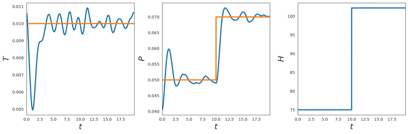
Plot NPT Results

Now, let’s plot the temperature as a function of time. We see that the temperature tracks the goal temperature with some fluctuations.

plt.subplot(1, 3, 1)

t = onp.arange(0, steps) * dt
plt.plot(t, log['kT'], linewidth=3)
plt.plot(t, kT * np.ones_like(t), linewidth=3)
plt.xlim([t[0], t[-1]])
format_plot('$t$', '$T$')

plt.subplot(1, 3, 2)

t = onp.arange(0, steps) * dt
plt.plot(t, log['P'], linewidth=3)
plt.plot(t, P(t), linewidth=3)
plt.xlim([t[0], t[-1]])
format_plot('$t$', '$P$')

plt.subplot(1, 3, 3)

t = onp.arange(0, steps) * dt
plt.plot(t, log['H'], linewidth=3)
plt.xlim([t[0], t[-1]])
format_plot('$t$', '$H$')

finalize_plot((2, 2 / 3))

Visualize Final State

Now let’s plot a snapshot of the system.

ms = 20 if SMOKE_TEST else 10
R_plt = onp.array(state.position)

plt.plot(R_plt[:N_2, 0], R_plt[:N_2, 1], 'o', markersize=ms * 0.5)
plt.plot(R_plt[N_2:, 0], R_plt[N_2:, 1], 'o', markersize=ms * 0.7)

plt.xlim([0, np.max(R[:, 0])])
plt.ylim([0, np.max(R[:, 1])])

plt.axis('off')

finalize_plot((2, 2))

Animation (Optional)

If we want, we can also draw an animation of the simulation using JAX MD’s renderer. This only works in Google Colab.

if IN_COLAB:
  from jax_md.colab_tools import renderer

  diameters = sigma[species, species]
  colors = np.where(
    species[:, None],
    np.array([[1.0, 0.5, 0.01]]),
    np.array([[0.35, 0.65, 0.85]]),
  )

  renderer.render(
    box[0, 0],
    {'particles': renderer.Disk(log['position'], diameters, colors)},
    buffer_size=20,
    resolution=(700, 700),
  )
else:
  print('Renderer only available in Google Colab. Skipping.')

Renderer only available in Google Colab. Skipping.

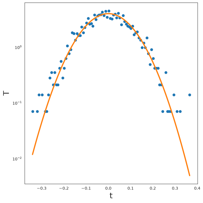
Velocity Distribution

Finally, let’s plot the velocity distribution compared with its theoretical prediction.

V_flat = onp.reshape(onp.array(state.velocity), (-1,))
occ, bins = onp.histogram(V_flat, bins=100, density=True)

T_cur = kT
plt.semilogy(bins[:-1], occ, 'o')
plt.semilogy(
  bins[:-1],
  1.0 / np.sqrt(2 * np.pi * T_cur) * onp.exp(-1 / (2 * T_cur) * bins[:-1] ** 2),
  linewidth=3,
)
format_plot('t', 'T')
finalize_plot()