Multi-Image Neighbor Lists for Small Periodic Boxes#
This tutorial demonstrates how to use multi-image neighbor lists in JAX-MD for systems where the cutoff radius is larger than half the box length (\(r_\text{cut} > L/2\)).
The Problem with Standard Neighbor Lists#
Standard neighbor lists in JAX-MD use the Minimum Image Convention (MIC), which assumes each atom interacts with at most one periodic image of every other atom. This works well when:
However, for small periodic boxes (common in ab initio MD or machine learning potentials with longer cutoffs), an atom may interact with multiple periodic images of the same neighbor. The multi-image neighbor list explicitly enumerates all images within the cutoff.
Imports & Setup#
[1]:
import os

IN_COLAB = 'COLAB_RELEASE_TAG' in os.environ
if IN_COLAB:
  import subprocess
  import sys

  subprocess.run(
    [
      sys.executable,
      '-m',
      'pip',
      'install',
      '-q',
      'git+https://github.com/jax-md/jax-md.git',
    ]
  )

import numpy as onp

from jax import config

config.update('jax_enable_x64', True)

import jax.numpy as jnp
from jax import random, jit, lax

import time
import matplotlib.pyplot as plt
import seaborn as sns

from jax_md import space, energy, partition, quantity, simulate
from jax_md.custom_partition import neighbor_list_multi_image
from jax_md.custom_smap import pair_neighbor_list_multi_image

SMOKE_TEST = os.environ.get('READTHEDOCS', False)

sns.set_style(style='white')


def format_plot(x, y):
  plt.xlabel(x, fontsize=20)
  plt.ylabel(y, fontsize=20)


def finalize_plot(shape=(1, 1)):
  plt.gcf().set_size_inches(
    shape[0] * 1.5 * plt.gcf().get_size_inches()[1],
    shape[1] * 1.5 * plt.gcf().get_size_inches()[1],
  )
  plt.tight_layout()
Matplotlib is building the font cache; this may take a moment.
Helper: Create Crystal Structures#
[2]:
def make_fcc(n_cells, a=1.0):
  """Create FCC crystal positions in fractional coordinates.

  Args:
    n_cells: Number of unit cells in each direction.
    a: Lattice constant.

  Returns:
    R: Fractional positions of shape [N, 3] in [0, 1).
    box: Box matrix of shape [3, 3] with columns as lattice vectors.
  """
  # FCC basis: 4 atoms per unit cell
  basis = onp.array(
    [
      [0.0, 0.0, 0.0],
      [0.5, 0.5, 0.0],
      [0.5, 0.0, 0.5],
      [0.0, 0.5, 0.5],
    ]
  )

  positions = []
  for i in range(n_cells):
    for j in range(n_cells):
      for k in range(n_cells):
        for b in basis:
          pos = (onp.array([i, j, k]) + b) / n_cells
          positions.append(pos)

  R = onp.array(positions)
  L = n_cells * a
  box = onp.eye(3) * L
  return jnp.array(R), jnp.array(box)


def make_diamond_cubic(n_cells, a=5.43):
  """Create diamond cubic crystal using the 2-atom primitive cell.

  Uses the FCC primitive cell with a 2-atom basis:
  - Lattice vectors: a1=(0,1,1)a/2, a2=(1,0,1)a/2, a3=(1,1,0)a/2
  - Basis: (0,0,0) and (1/4,1/4,1/4) in fractional coordinates

  This is more efficient than the 8-atom conventional cell.
  Used for silicon (a=5.43 Å) and germanium (a=5.66 Å).

  Args:
    n_cells: Number of primitive cells in each direction.
    a: Conventional cubic lattice constant (default 5.43 Å for silicon).

  Returns:
    R: Fractional positions of shape [N, 3] in [0, 1).
    box: Box matrix of shape [3, 3] with columns as FCC primitive vectors.
  """
  # 2-atom basis in fractional coordinates of primitive cell
  basis = onp.array(
    [
      [0.0, 0.0, 0.0],
      [0.25, 0.25, 0.25],
    ]
  )

  positions = []
  for i in range(n_cells):
    for j in range(n_cells):
      for k in range(n_cells):
        for b in basis:
          pos = (onp.array([i, j, k]) + b) / n_cells
          positions.append(pos)

  R = onp.array(positions)

  # FCC primitive lattice vectors (columns of box matrix)
  # a1 = (0, a/2, a/2), a2 = (a/2, 0, a/2), a3 = (a/2, a/2, 0)
  box = (a / 2.0) * onp.array(
    [
      [0.0, 1.0, 1.0],
      [1.0, 0.0, 1.0],
      [1.0, 1.0, 0.0],
    ]
  )
  # Scale by n_cells
  box = box * n_cells

  return jnp.array(R), jnp.array(box)
Example 1: Lennard-Jones with All Three neighbor list formats#
We compute LJ energy for a small FCC argon crystal using all three neighbor list formats to verify they produce identical results:
Dense: Per-atom neighbor arrays
[N, max_neighbors]Sparse: Edge list
[2, capacity]with both directionsOrderedSparse: Edge list with one direction per pair (most efficient)
[3]:
# Argon LJ parameters (reduced units: sigma=1, epsilon=1)
sigma = 1.0  # Length unit
epsilon = 1.0  # Energy unit
r_cutoff = 2.5 * sigma
r_onset = 2.0 * sigma

# Create small FCC argon crystal where r_cut > L/2
# In reduced units, equilibrium nearest-neighbor distance ≈ 2^(1/6) * sigma ≈ 1.12
# FCC lattice constant a = sqrt(2) * nearest_neighbor ≈ 1.58 in reduced units
n_cells = 2
a_reduced = 1.55  # Small box to test multi-image (r_cut/L > 0.5)
R, box = make_fcc(n_cells, a=a_reduced)
N = len(R)
L = float(box[0, 0])

print(f'System: {N} Ar atoms in {n_cells}x{n_cells}x{n_cells} FCC')
print(f'Box size L = {L:.2f}sigma, r_cutoff = {r_cutoff:.2f}sigma')
print(f'r_cutoff / L = {r_cutoff / L:.2f} (> 0.5: multi-image needed)')

# Setup displacement function
displacement_fn, shift_fn = space.periodic_general(
  box, fractional_coordinates=True
)

# Test all three formats
formats = [
  ('Dense', partition.Dense),
  ('Sparse', partition.Sparse),
  ('OrderedSparse', partition.OrderedSparse),
]

energies = {}
for name, fmt in formats:
  neighbor_fn, energy_fn = energy.lennard_jones_neighbor_list(
    displacement_fn,
    box,
    sigma=sigma,
    epsilon=epsilon,
    r_onset=r_onset / sigma,
    r_cutoff=r_cutoff / sigma,
    fractional_coordinates=True,
    neighbor_list_fn=neighbor_list_multi_image,
    pair_neighbor_list_fn=pair_neighbor_list_multi_image,
    format=fmt,
  )

  nbrs = neighbor_fn.allocate(R)
  E = float(energy_fn(R, nbrs))
  energies[name] = E

  # Get neighbor count
  if partition.is_sparse(fmt):
    n_edges = int(jnp.sum(nbrs.idx[0] < N))
  else:
    n_edges = int(jnp.sum(nbrs.idx < N))

  print(f'{name:15s}: E = {E:12.6f}, edges = {n_edges}')

# Verify all formats give the same energy
E_ref = energies['Dense']
for name, E in energies.items():
  assert abs(E - E_ref) < 1e-5, f'{name} energy mismatch: {E} vs {E_ref}'
System: 32 Ar atoms in 2x2x2 FCC
Box size L = 3.10sigma, r_cutoff = 2.50sigma
r_cutoff / L = 0.81 (> 0.5: multi-image needed)
Dense          : E =  -250.355417, edges = 4288
/home/docs/checkouts/readthedocs.org/user_builds/jax-md/envs/main/lib/python3.12/site-packages/jax/_src/ops/scatter.py:104: FutureWarning: scatter inputs have incompatible types: cannot safely cast value from dtype=int64 to dtype=int32 with jax_numpy_dtype_promotion=standard. In future JAX releases this will result in an error.
  warnings.warn(
Sparse         : E =  -250.355417, edges = 4288
OrderedSparse  : E =  -250.355417, edges = 2144
Forces and Stress Computation#
We can compute forces using quantity.force and stress using quantity.stress. The multi-image neighbor list with graph_featurizer supports the perturbation kwarg required for stress calculation.
[4]:
# Use Sparse format for force/stress computation
neighbor_fn_lj, energy_fn_lj = energy.lennard_jones_neighbor_list(
  displacement_fn,
  box,
  sigma=sigma,
  epsilon=epsilon,
  r_onset=r_onset / sigma,
  r_cutoff=r_cutoff / sigma,
  fractional_coordinates=True,
  neighbor_list_fn=neighbor_list_multi_image,
  pair_neighbor_list_fn=pair_neighbor_list_multi_image,
  format=partition.Sparse,
)

# Perturb positions slightly from equilibrium to get non-zero forces
key = random.PRNGKey(42)
R_perturbed = R + random.normal(key, R.shape) * 0.01

nbrs_lj = neighbor_fn_lj.allocate(R_perturbed)
E_lj = float(energy_fn_lj(R_perturbed, nbrs_lj))

# Compute forces
force_fn = quantity.force(energy_fn_lj)
F = force_fn(R_perturbed, neighbor=nbrs_lj)
max_force = float(jnp.max(jnp.abs(F)))
print(f'Perturbed energy: {E_lj:.6f}')
print(f'Max force magnitude: {max_force:.6f}')

# Compute stress (3x3 tensor)
stress = quantity.stress(energy_fn_lj, R_perturbed, box, neighbor=nbrs_lj)
print(f'Stress tensor (diagonal): [{stress[0,0]:.4f}, {stress[1,1]:.4f}, {stress[2,2]:.4f}]')
print(f'Pressure: {-jnp.trace(stress) / 3:.6f}')
Perturbed energy: -232.244742
Max force magnitude: 51.575608
Stress tensor (diagonal): [2.8778, 3.3587, 3.1045]
Pressure: -3.113656
Example 2: Stillinger-Weber (Three-Body Potential)#
Stillinger-Weber is a three-body potential for silicon that requires Dense format for the angular terms. We use a 2x2x2 supercell of the 2-atom primitive cell.
Note: Stillinger-Weber internally uses space.map_neighbor for displacement computation, which applies the minimum image convention (MIC). For small boxes where r_cut > L/2, the multi-image neighbor list finds the correct neighbors, but the energy computation would still use MIC displacements. Therefore, we use a larger box where MIC is valid.
[5]:
# Stillinger-Weber parameters for silicon
sw_sigma = 2.0951  # Angstrom
sw_cutoff = 1.8 * sw_sigma  # ~3.77 Angstrom

# Create 3x3x3 supercell so that MIC is valid
# For SW, the box must be large enough that r_cut < L/2
n_cells_sw = 3
a_sw = 5.43  # Si lattice constant
R_sw, box_sw = make_diamond_cubic(n_cells_sw, a=a_sw)
N_sw = len(R_sw)

# For non-cubic boxes, compute minimum perpendicular height
inv_box_T = jnp.linalg.inv(box_sw).T
heights_sw = 1.0 / jnp.linalg.norm(inv_box_T, axis=0)
L_min_sw = float(jnp.min(heights_sw))

print(f'System: {N_sw} Si atoms in {n_cells_sw}x{n_cells_sw}x{n_cells_sw} diamond cubic supercell')
print(f'Min box height = {L_min_sw:.2f} Angstrom, SW cutoff = {sw_cutoff:.2f} Angstrom')
print(f'cutoff / L_min = {sw_cutoff / L_min_sw:.2f} (< 0.5: MIC is valid)')

displacement_sw, shift_sw = space.periodic_general(
  box_sw, fractional_coordinates=True
)

# Stillinger-Weber only supports Dense format (three-body terms)
# Note: SW uses MIC internally, so multi-image NL only helps with neighbor finding
neighbor_fn_sw, energy_fn_sw = energy.stillinger_weber_neighbor_list(
  displacement_sw,
  box_sw,
  neighbor_list_fn=neighbor_list_multi_image,
  format=partition.Dense,
  fractional_coordinates=True,
)

nbrs_sw = neighbor_fn_sw.allocate(R_sw)
E_sw = float(energy_fn_sw(R_sw, nbrs_sw))
n_edges_sw = int(jnp.sum(nbrs_sw.idx < N_sw))

print(f'Stillinger-Weber energy: {E_sw:.6f} eV')
print(f'Number of edges: {n_edges_sw}')
print('Stillinger-Weber computes correctly (MIC valid for this box size).')
System: 54 Si atoms in 3x3x3 diamond cubic supercell
Min box height = 9.41 Angstrom, SW cutoff = 3.77 Angstrom
cutoff / L_min = 0.40 (< 0.5: MIC is valid)
Stillinger-Weber energy: -234.171986 eV
Number of edges: 864
Stillinger-Weber computes correctly (MIC valid for this box size).
Example 3: NVE Molecular Dynamics#
We run NVE (constant energy) molecular dynamics with the multi-image neighbor list. This demonstrates rebuild tracking and overflow handling following the pattern recommended in partition.neighbor_list documentation.
[6]:
# Simulation parameters
N_md = 500
dimension = 2
box_size = 40.0 if SMOKE_TEST else 60.0

# Create box matrix for 2D
box_md = jnp.eye(dimension) * box_size

# Random initial positions (fractional coordinates in [0, 1))
key = random.PRNGKey(0)
R_md = random.uniform(key, (N_md, dimension), minval=0.0, maxval=1.0)

# 50:50 mixture of two species
sigma_md = jnp.array([[1.0, 1.2], [1.2, 1.4]])
N_half = N_md // 2
species = jnp.where(jnp.arange(N_md) < N_half, 0, 1)

# Cutoff
r_cutoff_md = 2.5

print(f'System: {N_md} atoms in {dimension}D box of size {box_size}')
print(f'Cutoff: {r_cutoff_md}, cutoff/L = {r_cutoff_md / box_size:.3f}')

# Setup displacement function for fractional coordinates
displacement_md, shift_md = space.periodic_general(
  box_md, fractional_coordinates=True
)

# For random positions, use generous capacity to avoid overflow
# Random positions can cluster, requiring more capacity than uniform estimates

# Use soft sphere potential with multi-image neighbor list
neighbor_fn_md, energy_fn_md = energy.soft_sphere_neighbor_list(
  displacement_md,
  box_md,
  species=species,
  sigma=sigma_md,
  fractional_coordinates=True,
  neighbor_list_fn=neighbor_list_multi_image,
  pair_neighbor_list_fn=pair_neighbor_list_multi_image,
  format=partition.Sparse,
)

# Initialize neighbor list
nbrs_md = neighbor_fn_md.allocate(R_md)
if nbrs_md.did_buffer_overflow:
  raise RuntimeError('Neighbor list overflowed - increase max_neighbors')

# Setup NVE integrator
dt = 1e-2
init_fn, apply_fn = simulate.nve(energy_fn_md, shift_md, dt)

# Initialize state with zero temperature
state = init_fn(key, R_md, neighbor=nbrs_md, kT=0.0)


# JIT-compiled step function with neighbor list update
@jit
def step_fn(i, state_and_nbrs):
  state, nbrs = state_and_nbrs
  state = apply_fn(state, neighbor=nbrs)
  nbrs = nbrs.update(state.position)
  return state, nbrs
System: 500 atoms in 2D box of size 40.0
Cutoff: 2.5, cutoff/L = 0.062
[7]:
# Run simulation following JAX-MD's recommended pattern for overflow handling.
# See partition.neighbor_list docstring for the canonical example.
N_steps = 200 if SMOKE_TEST else 1000
print_every = 20
inner_steps = 10

PE = []
KE = []
rebuild_count = 0
realloc_count = 0

print(f'{"Step":>4} {"KE":>5} {"PE":>6} {"Total":>6} {"dt":>6} {"rebuild":>7} {"realloc":>7}')
old_time = time.time()

for i in range(N_steps):
  # Track reference position before inner loop
  old_ref_pos = nbrs_md.reference_position

  # Run inner_steps using fori_loop for efficiency
  new_state, new_nbrs = lax.fori_loop(0, inner_steps, step_fn, (state, nbrs_md))

  # Check for buffer overflow after the loop
  # If overflow: discard new state, reallocate with extra capacity
  # If no overflow: accept new state
  if new_nbrs.did_buffer_overflow:
    # Reallocate with extra capacity (10 more neighbors per atom)
    nbrs_md = neighbor_fn_md.allocate(state.position, extra_capacity=10)
    realloc_count += 1
    print(f'  [Overflow at step {i * inner_steps}! Reallocating with extra capacity...]')
    # Don't advance state - retry from last good state
  else:
    # Accept the new state
    state = new_state
    nbrs_md = new_nbrs

    # Check if rebuild happened (reference position changed)
    new_ref_pos = nbrs_md.reference_position
    if not jnp.allclose(old_ref_pos, new_ref_pos):
      rebuild_count += 1

  pe = float(energy_fn_md(state.position, nbrs_md))
  ke = float(quantity.kinetic_energy(momentum=state.momentum))
  PE.append(pe)
  KE.append(ke)

  if i % print_every == 0 and i > 0:
    new_time = time.time()
    step_time = (new_time - old_time) / print_every / inner_steps
    print(
      f'{i * inner_steps:4d} {ke:5.1f} {pe:6.1f} {ke + pe:6.2f} '
      f'{step_time:6.4f} {rebuild_count:7d} {realloc_count:7d}'
    )
    old_time = new_time

PE = jnp.array(PE)
KE = jnp.array(KE)

print(f'Total energy drift: {abs(float(PE[-1] + KE[-1] - PE[0] - KE[0])):.2e}')
print(f'Total rebuilds: {rebuild_count}, reallocs: {realloc_count}')
Step    KE     PE  Total     dt rebuild realloc
 200  26.3    5.5  31.75 0.0223      16       0
 400  27.0    4.8  31.75 0.0136      34       0
 600  26.8    4.9  31.74 0.0141      51       0
 800  26.8    5.0  31.74 0.0131      68       0
1000  25.5    6.3  31.74 0.0141      88       0
1200  27.4    4.4  31.74 0.0138     107       0
1400  25.7    6.1  31.75 0.0140     126       0
1600  26.0    5.8  31.75 0.0154     145       0
1800  26.4    5.4  31.75 0.0127     162       0
Total energy drift: 9.10e-03
Total rebuilds: 178, reallocs: 0
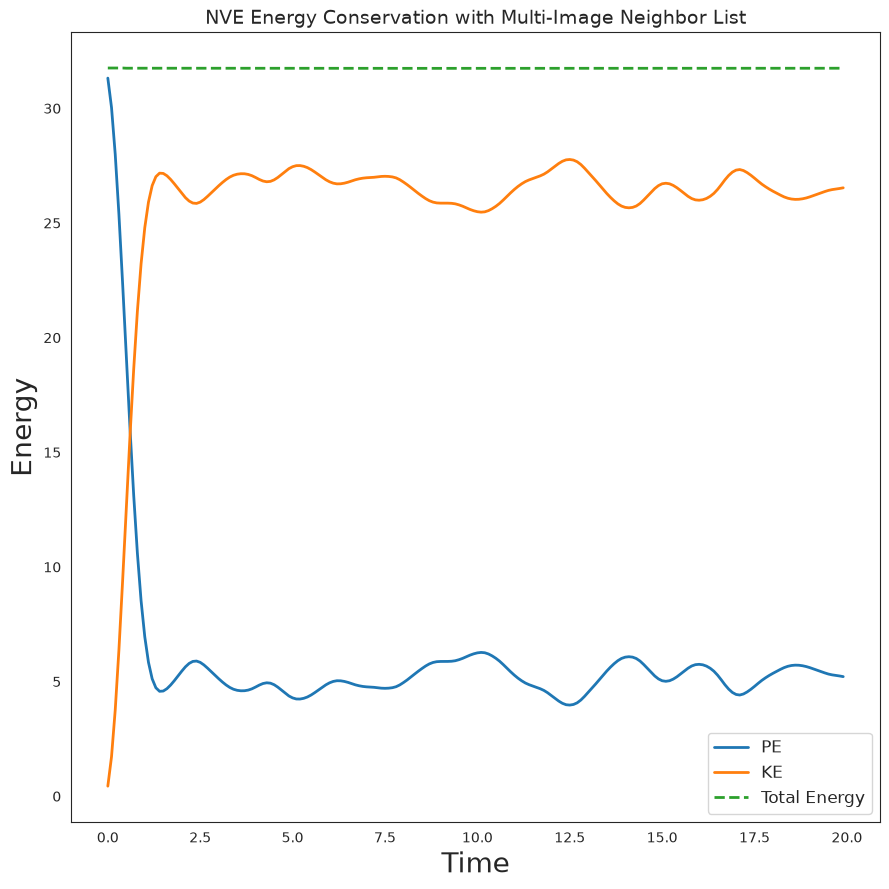
Plot Energy Evolution#
We verify energy conservation by plotting PE, KE, and total energy over time.
[8]:
t = onp.arange(N_steps) * dt * inner_steps

plt.figure(figsize=(10, 6))
plt.plot(t, PE, label='PE', linewidth=2)
plt.plot(t, KE, label='KE', linewidth=2)
plt.plot(t, PE + KE, label='Total Energy', linewidth=2, linestyle='--')
plt.legend(fontsize=12)
format_plot('Time', 'Energy')
plt.title('NVE Energy Conservation with Multi-Image Neighbor List', fontsize=14)
finalize_plot()
plt.savefig('nve_multi_image.png', dpi=150, bbox_inches='tight')
plt.show()
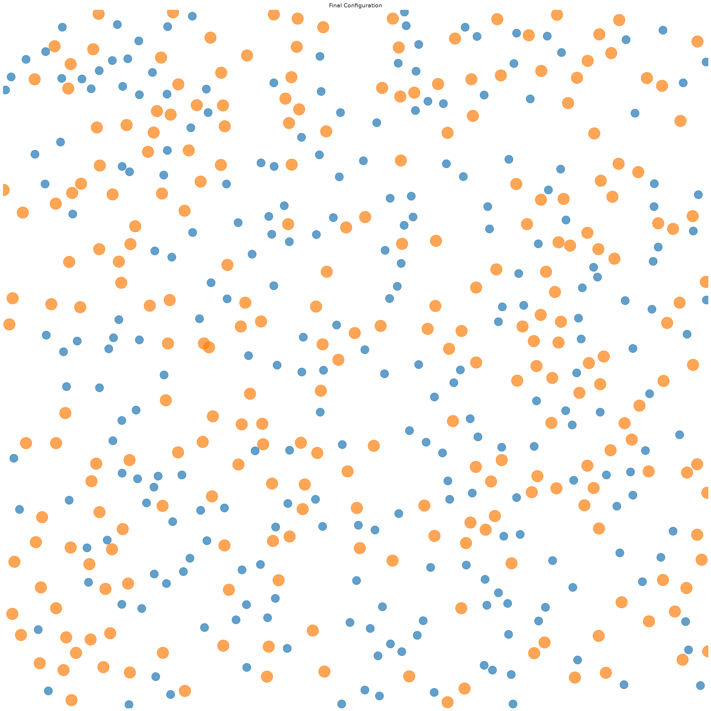
Visualize Final Configuration#
[9]:
ms = 40 if SMOKE_TEST else 15
R_final = onp.array(state.position)

# Convert from fractional to Cartesian for plotting
R_cart = R_final * box_size

plt.figure(figsize=(8, 8))
plt.plot(
  R_cart[:N_half, 0], R_cart[:N_half, 1], 'o', markersize=ms * 0.5, alpha=0.7
)
plt.plot(
  R_cart[N_half:, 0], R_cart[N_half:, 1], 'o', markersize=ms * 0.7, alpha=0.7
)
plt.xlim([0, box_size])
plt.ylim([0, box_size])
plt.axis('off')
plt.title('Final Configuration', fontsize=14)
finalize_plot((2, 2))
plt.savefig('nve_final_config.png', dpi=150, bbox_inches='tight')
plt.show()